Introduction
There are three main legend-related function groups in ggplots:
guides(), scale_XX family of functions, and
theme(). In my previous posts, I showed how we can modify
discrete and continuous legends using the first two function groups
(check theme out here! Post
#10, Post
#11, Post
#16, and Post
#17). In this post, I will continue to introduce to you the third
function “theme()”. I’ll also wrap up this topic by
summarizing the features of these three function groups and discuss
their usages. After this journey, I believe you will be able to make the
most of these functions to achieve your ggplot goals!
The theme() function
theme() is one of the key components of ggplots and
controls various aspects of the plot appearance: plot title, panel
background, axis labels, grid lines, facet strips, and of course
legends. There are quite a few legend-related arguments in
theme(). To make life easier, I classify them into four
main categories based on which parts of the legends they focus on:
(1) Arguments for legend box (2) Arguments for legend keys (3) Arguments for legend title and labels (4) Arguments for legend layout
Let’s kick things off by creating an example plot with two legends,
one discrete and one continuous, using the CO2
data set:
library(tidyverse)

P <- ggplot(data = CO2) +
  geom_boxplot(aes(x = Treatment, y = uptake, color = Treatment), width = 0.5) +
  geom_point(aes(x = Treatment, y = uptake, fill = uptake), position = position_jitter(width = 0.05), shape = 21, size = 2, color = "transparent") +
  labs(x = "Treatment", y = expression(paste(CO[2], " uptake rate"))) +
  theme_classic(base_size = 14) +
  scale_color_brewer(palette = "Set1") +
  scale_fill_viridis_c(name = expression(paste(CO[2], " uptake rate")))

P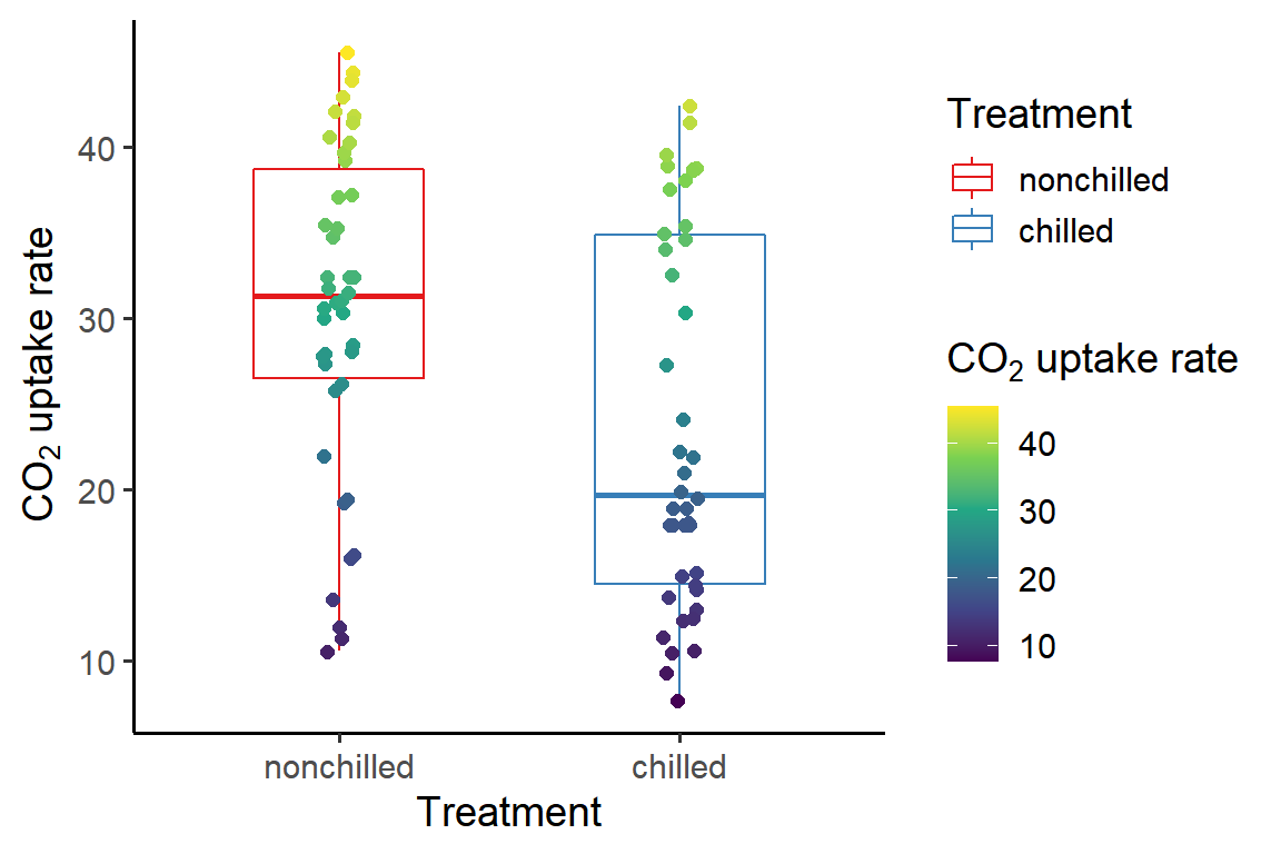
(1) Arguments for legend box
These arguments control the appearance and margin of entire legend area as well as individual legend boxes, the arrangement of multiple legends, and the spacing between panel area and legend area:
P + theme(# the appearance of entire legend area
          legend.box.background = element_rect(fill = "green1",
                                               color = "black",
                                               size = 1,
                                               linetype = "dashed"),

          # the margin of entire legend area
          legend.box.margin = margin(t = 50, r = 10, b = 50, l = 10),

          # the appearance of individual legend boxes
          legend.background = element_rect(fill = "grey90",
                                           color = "black",
                                           size = 0.5,
                                           linetype = "dotted"),

          # the margin of individual legend boxes
          legend.margin = margin(t = 5, r = 15, b = 5, l = 15),

          # the arrangement of the legends
          legend.box = "horizontal",
          legend.box.just = "right",

          # the spacing between panel area and legend area
          legend.box.spacing = unit(0, "inch"))
Did you notice that both legends were modified in the same manner?
This is an important feature of theme(): it changes
everything in the plot (i.e., global effect)! So if you want to
modify just a certain legend, or modify the legends differently (i.e.,
local effect), you should use guides() instead and specify
a specific legend (e.g., the legend for “color” aesthetics) to
modify.
(2) Arguments for legend keys
These arguments control the appearance and size (height and width) of legend keys:
P + theme(# the appearance of legend keys
          legend.key = element_rect(fill = "orange",
                                    color = "black",
                                    size = 0.5,
                                    linetype = "solid"),

          # the height of legend keys
          legend.key.height = unit(0.3, "inch"),

          # the width of legend keys
          legend.key.width = unit(0.6, "inch"))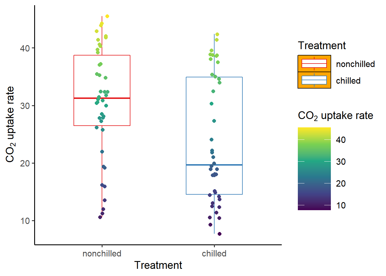
(3) Arguments for legend title and labels
These arguments control the appearance and alignment of legend title and labels, the spacing between legend keys and labels, and the spacing between legend title and keys/labels:
P + theme(# the appearance of legend title
          legend.title = element_text(size = 15,
                                      margin = margin(l = -10)),

          # the alignment of legend title
          legend.title.align = 0.5,

          # the appearance of legend labels
          legend.text = element_text(color = "red",
                                     face = "bold",
                                     angle = 45),

          # the alignment of legend labels
          legend.text.align = 0.5,

          # the spacing between legend keys and labels
          legend.spacing.x = unit(0.5, "inch"),

          # the spacing between legend title and keys/labels
          legend.spacing.y = unit(0.2, "inch"))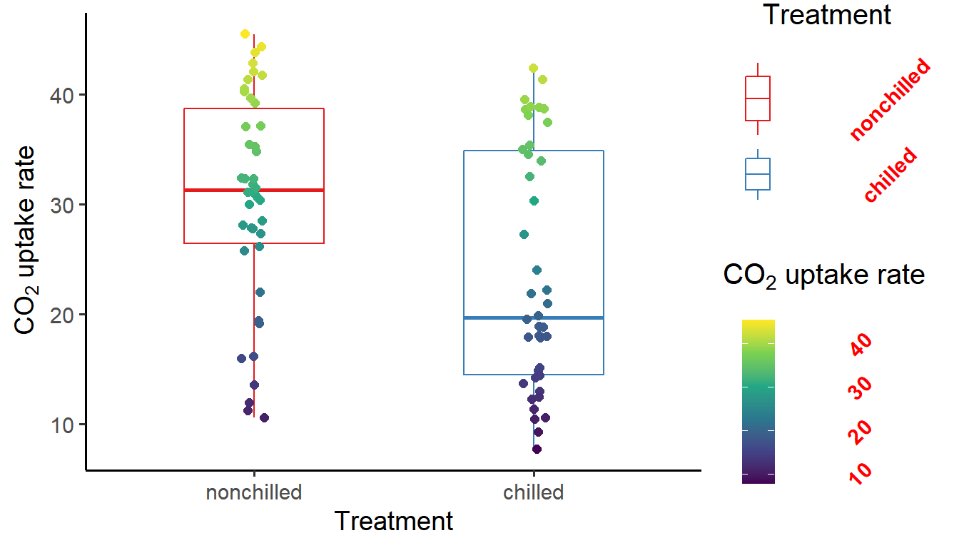
In the above figure, I centered the long title “CO2 uptake rate” by specifying a negative left margin, which pulled the title to the left. Check out my very first post on this trick if interested!
(4) Arguments for legend layout
These arguments control the position of legend area and the direction of legend items:
P + theme(# the position of legend area
          legend.position = "top",  # can pass a vector c(x, y) as well

          # the direction of legend items
          legend.direction = "horizontal")
For the argument legend.position, besides the built-in
positions (“top”, “right”, “bottom”, “left”), you can also place the
legend(s) inside the plot by passing a vector of length two
c(x, y) (between 0 and 1) as the x- and y-coordinate
relative to the plot area. For instance,
legend.position = c(0.5, 0.5) will place the legend(s) in
the middle of the plot.
Comparisons of the three function groups
Here is a summary table of the key features of the three legend-related function groups:
| guides() | scale_XX functions | theme() | |
|---|---|---|---|
| General appearance of legends | X | X | |
| Arrangement/layout of legends | X | X | |
| Scales (e.g., range) of legends | X | ||
| Text of legend title/labels | X | ||
| Order of legend keys | X | ||
| Override default legend keys | X | ||
| Effect | Local | Local | Global |
In general, guides() and theme() resemble
each other and both control the physical appearance of legends, whereas
scale_XX functions control the scales (legend range, legend
tick positions, etc.) and text (the words displayed in title and labels)
of legends. Additionally, there are some specific legend modifications
that certain functions can make. For example, scale_XX
functions can be used to reorder the legend items; guides()
can be used to overwrite the default aesthetic mappings of legend keys.
Finally, these three functions differ in their effects:
theme() affects every legend in the plot, whereas
guides() and scale_XX functions affect only
the specified legend(s).
Summary
In this post, I showed how you can use various theme()
arguments to modify the appearance of ggplot legends: legend box, legend
keys, legend title and labels, and legend layout. I also summarized the
features of three legend-related function groups (guides(),
scale_XX, and theme()) and offered some tips
for using them. Of course, having a combination of these functions is
the best way to achieve the desired outcome!
Hope you learn something useful from this post and don’t forget to leave your comments and suggestions below if you have any!
