In this post, we will be working on continuous legends in ggplots with guides(). This is a continuation of the previous post on discrete legends. Check it out here if you haven’t!
Continuous legends
As mentioned in the previous post, there are two main types of legends in ggplots: discrete and continuous. The former corresponds to the aesthetics mapped to categorical variables (e.g., gender and eye color), whereas the latter corresponds to the aesthetics mapped to continuous variables (e.g., tree height and population density).
Instead of using built-in datasets as before, this time we will create a dataset ourselves by drawing random numbers from normal distributions (with various means but a fixed standard deviation of 1) for x- and y-coordinates, and then we’ll visualize the 2D density distribution in a contour plot.
library(tidyverse)

### Random numbers from normal distributions
set.seed(123)
x_mean <- c(-2, 2.4, 1)
y_mean <- c(-1.3, -1, 2)
rand_df <- data.frame(x = unlist(map(x_mean, function(x){rnorm(n = 200, mean = x, sd = 1)})),
                      y = unlist(map(y_mean, function(x){rnorm(n = 200, mean = x, sd = 1)})))

### Contour plot
P <- ggplot(rand_df) +
  stat_density_2d(aes(x = x, y = y, fill = ..level..), geom = "polygon") +
  theme_classic(base_size = 14) +
  coord_fixed(ratio = 1) +
  scale_fill_gradientn(colors = terrain.colors(10))

P
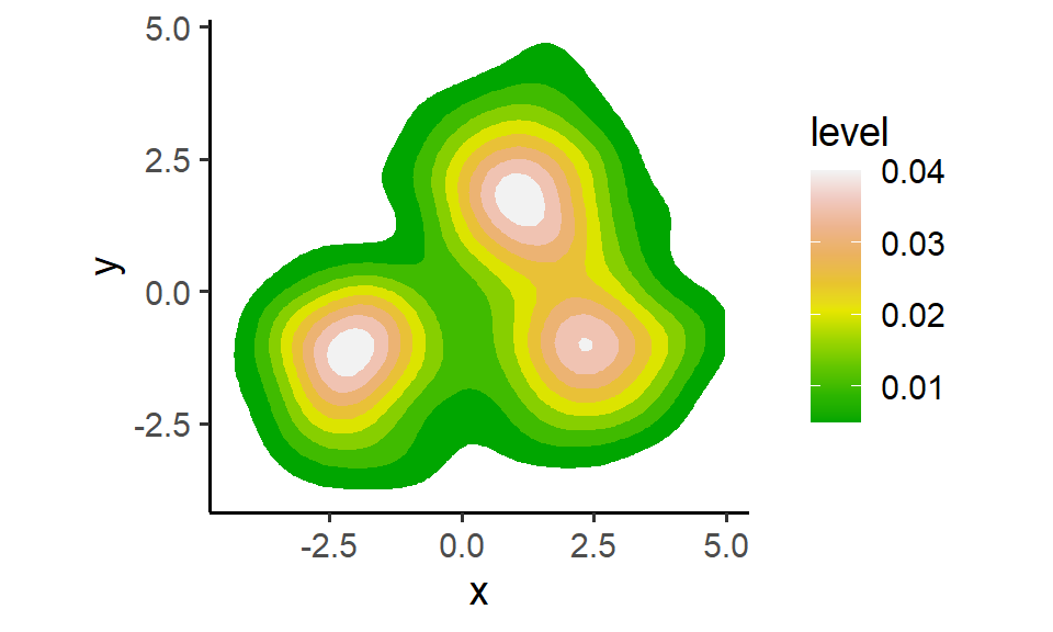
Here, the 2D kernel density estimate ..level.., an internal variable computed for the supplied data by stat_density_2d(), was mapped to the “fill” aesthetic as a continuous variable, and the contours were drawn using geom = "polygon".
The guide_colorbar() function
The actual function in guides() that controls the continuous legends is guide_colorbar(). In this example, we mapped the variable “..level..” to fill, so we will pass fill = guide_colorbar() into guides() and specify the arguments.
There are several things we can modify in the legend:
(1) Legend title (2) Legend labels (3) Legend bar (4) Legend layout
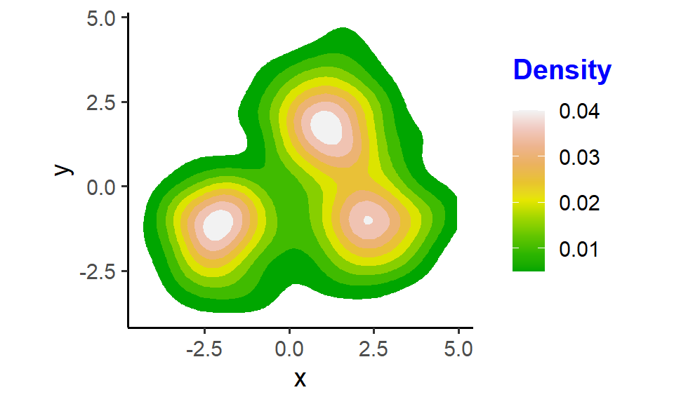
(1) Legend title
We can modify the name, position (relative to the legend labels and bar), and text appearance of the title. We can also adjust its horizontal and vertical alignment.
P + guides(fill = guide_colorbar(title = "Density",  # name
                                 title.position = "top",  # position
                                 title.theme = element_text(size = 15, color = "blue", face = "bold"),  # text appearance
                                 title.hjust = 0.5,  # horizontal alignment
                                 title.vjust = 3))  # vertical alignment
(2) Legend labels
Similarly, we can modify the position (relative to the legend bar) and text appearance of the labels as well as adjust the horizontal and vertical alignment. If we want to hide the labels, specify label = F.
P + guides(fill = guide_colorbar(label = T,  # show the labels
                                 label.position = "left",  # position
                                 label.theme = element_text(size = 12, color = "brown", face = "italic"),  # text appearance
                                 label.hjust = 0,  # horizontal alignment
                                 label.vjust = 0.5))  # vertical alignment

(3) Legend bar
We can change the width and height of the legend bar to make the color gradient more discernible. We can also modify the appearance of bar frame and bar ticks.
P + guides(fill = guide_colorbar(barwidth = unit(0.2, "inches"),  # bar width
                                 barheight = unit(2, "inches"),  # bar height
                                 frame.colour = "black",  # bar frame color
                                 frame.linewidth = 2,  # bar frame width
                                 frame.linetype = "solid",  # bar frame linetype
                                 ticks = T,  # show the ticks on the bar
                                 ticks.linewidth = 2,  # tick width
                                 ticks.colour = "red",  # tick color
                                 draw.ulim = T,  # show the tick at the upper limit
                                 draw.llim = T  # show the tick at the lower limit
                                 ))

(4) Legend layout
We can display the legend either horizontally or vertically and flip the bar if needed.
P + guides(fill = guide_colorbar(direction = "horizontal",  # direction of the legend
                                 reverse = T))  # flip the bar

Summary
In this post, we’ve learned how to modify the appearance and layout of legend bar in continuous ggplot legends using the function guides(). Play around with the arguments a bit and I believe you will be able to make a nice legend(s) for your figure!
Hope you enjoy the reading and don’t forget to leave your comments and suggestions below if you have any!
