Before we start
“Blogenesis”! This is the origin of my first ggGallery blog post! Feel excited to write about something in which I am interested. This very first post is a simple one, but I bet it will be pretty handy. Hope you learn something from this post. Most importantly, enjoy the reading!
The problem
When making a ggplot with legend, the legend title is left-aligned by default:
library(tidyverse)

ggplot(mtcars, aes(wt, mpg)) +
  geom_point(aes(colour = factor(cyl))) +
  geom_smooth(aes(colour = factor(cyl)), method = "lm", se = F) +
  scale_color_discrete(name = "Cyl",
                       label = c("Four", "Six", "Eight")) +
  theme_classic(base_size = 13)
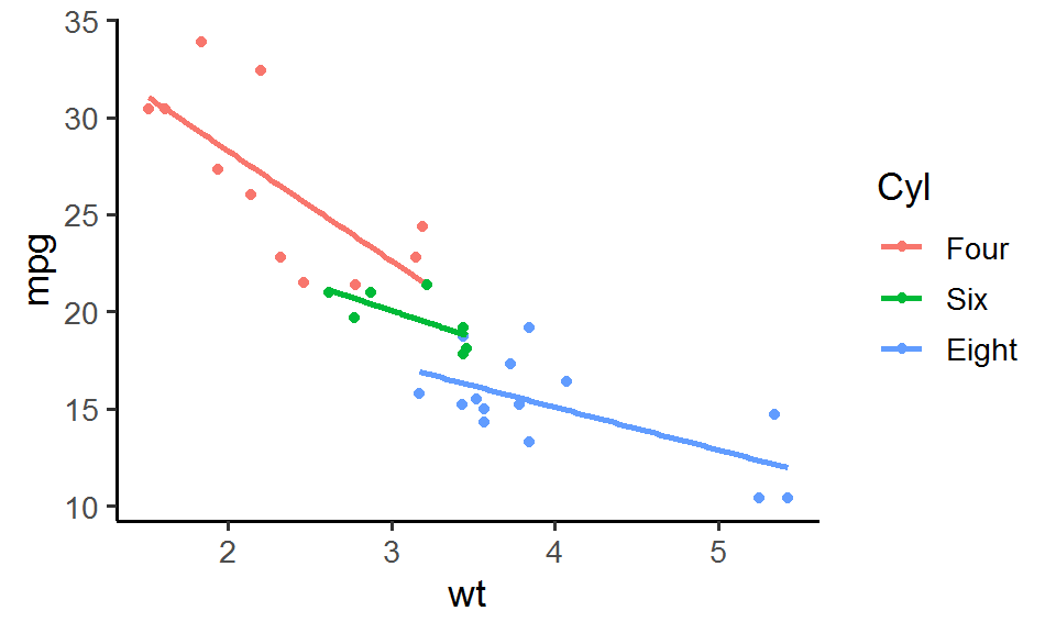
If you are happy with it, then fine. But oftentimes, we would like to align the legend title to the center so that the legend looks more balanced. For short titles, this is easy to achieve, just use theme(legend.title.align = 0.5):
ggplot(mtcars, aes(wt, mpg)) +
  geom_point(aes(colour = factor(cyl))) +
  geom_smooth(aes(colour = factor(cyl)), method = "lm", se = F) +
  scale_color_discrete(name = "Cyl",
                       label = c("Four", "Six", "Eight")) +
  theme_classic(base_size = 13) +
  theme(legend.title.align = 0.5) # Align the title to the center
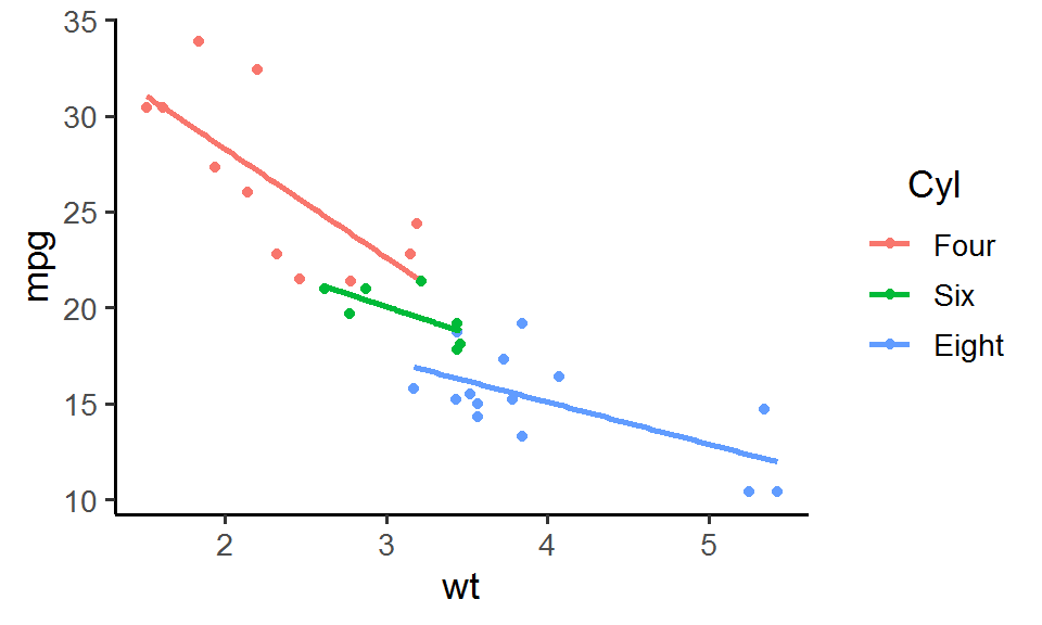
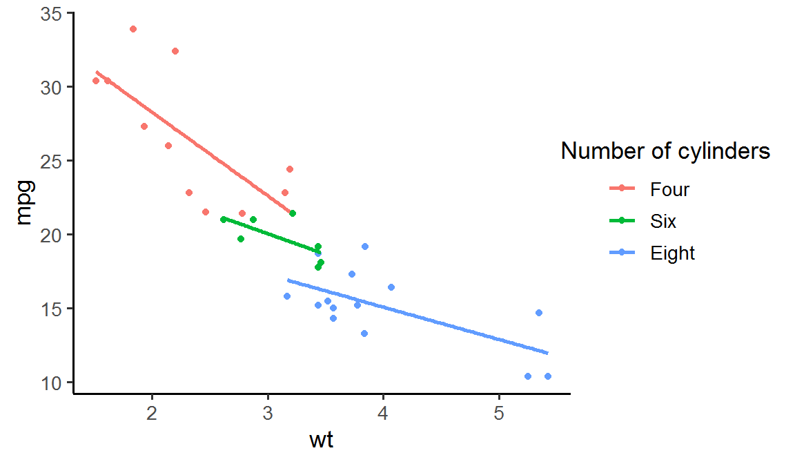
However, for legend titles that are longer than the legend keys and labels, this method does not work:
ggplot(mtcars, aes(wt, mpg)) +
  geom_point(aes(colour = factor(cyl))) +
  geom_smooth(aes(colour = factor(cyl)), method = "lm", se = F) +
  scale_color_discrete(name = "Number of cylinders",
                       label = c("Four", "Six", "Eight")) +
  theme_classic(base_size = 13) +
  theme(legend.title.align = 0.5) # Not work!

There is a solution to this problem on stackoverflow. Basically, what it does is to extract the individual elements from the legend grobs, add extra space, and finally piece them back together. This method really delves into the heart of ggplots, but such “brute force” method might require quite a bit of time as well as decent understandings of how ggplot legends is built.
So isn’t there a simpler and more elegant way to do so?
The hack
The answer to this question is a complete no-brainer: Yes! Otherwise, I will not be writing this blog, right?! Here is the hack: just use “negative” left margin around the legend title:
ggplot(mtcars, aes(wt, mpg)) +
  geom_point(aes(colour = factor(cyl))) +
  geom_smooth(aes(colour = factor(cyl)), method = "lm", se = F) +
  scale_color_discrete(name = "Number of cylinders",
                       label = c("Four", "Six", "Eight")) +
  theme_classic(base_size = 13) +
  theme(legend.title = element_text(margin = margin(l = -25))) # Negative left margin
Now the title lies nicely in the center of the legend. Hooray!
The explanation
So how does negative margin work? Let’s visualize it by showing the legend box border. By default, there is no margin around the title, which will fit just right within the box border:
# Default left margin
ggplot(mtcars, aes(wt, mpg)) +
  geom_point(aes(colour = factor(cyl))) +
  geom_smooth(aes(colour = factor(cyl)), method = "lm", se = F) +
  scale_color_discrete(name = "Number of cylinders",
                       label = c("Four", "Six", "Eight")) +
  theme_classic(base_size = 13) +
  theme(legend.title = element_text(margin = margin(l = 0)),
        legend.background = element_rect(color = "black")) +
  labs(title = "Default margin")
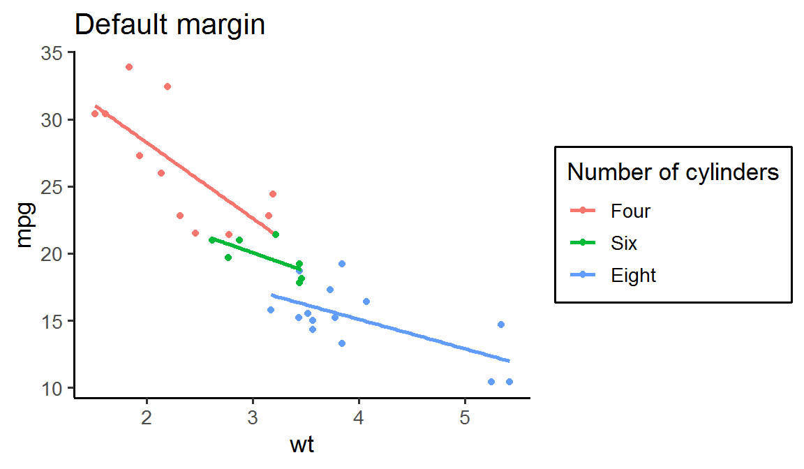
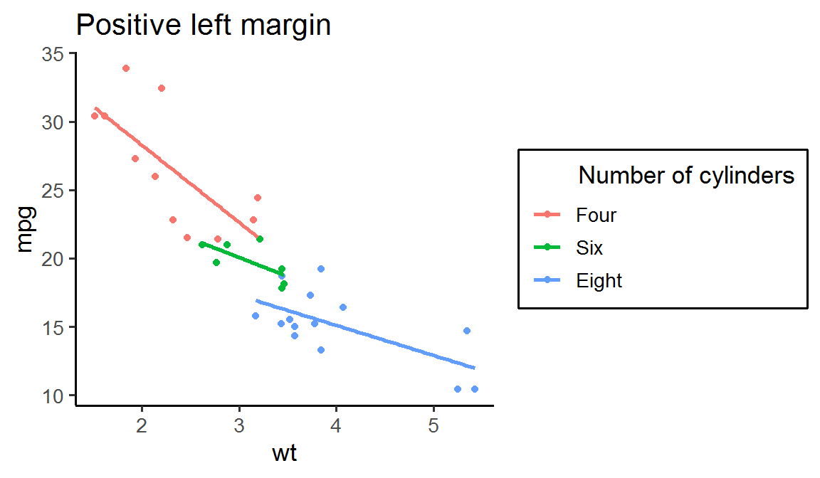
If you specify a positive left margin, then there will be extra space added between the title and left box border:
# Positive left margin
ggplot(mtcars, aes(wt, mpg)) +
  geom_point(aes(colour = factor(cyl))) +
  geom_smooth(aes(colour = factor(cyl)), method = "lm", se = F) +
  scale_color_discrete(name = "Number of cylinders",
                       label = c("Four", "Six", "Eight")) +
  theme_classic(base_size = 13) +
  theme(legend.title = element_text(margin = margin(l = 25)),
        legend.background = element_rect(color = "black")) +
  labs(title = "Positive left margin")
But if you specify a negative margin, then you are asking ggplot to add some “negative” space between the title and left box border, and what that means is that ggplot will “pull” the title toward left beyond the box border:
# Negative left margin
ggplot(mtcars, aes(wt, mpg)) +
  geom_point(aes(colour = factor(cyl))) +
  geom_smooth(aes(colour = factor(cyl)), method = "lm", se = F) +
  scale_color_discrete(name = "Number of cylinders",
                       label = c("Four", "Six", "Eight")) +
  theme_classic(base_size = 12) +
  theme(legend.title = element_text(margin = margin(l = -25)),
        legend.background = element_rect(color = "black")) +
  labs(title = "Negative left margin")
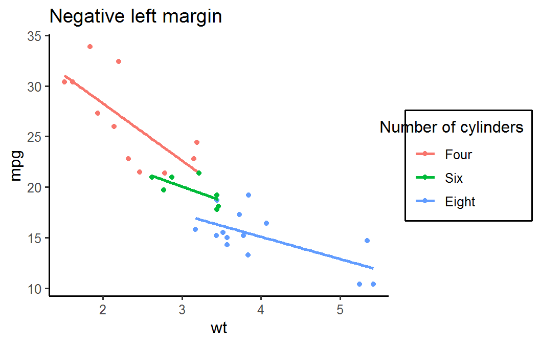
And after removing the box border, you will find that the title just moves to the center of the legend!
Finally, I think you might ask: what negative margin value should I specify? The answer is: it depends! It really depends on the relative length of your title to your legend keys and labels, and so you might need to try out a few different values and see how it goes. Though this might seem a bit tedious, it offers you the most flexibility to place your title at the exact position you desire. It is worth the effort!
Definitely try this tip out next time. And if you have any further ideas or questions, don’t forget to leave them below!
