Welcome to the first post of 2022—also my 10th ggGallery post! A tiny but meaningful milestone reached!
Background
Legends are arguably one of the greatest advantages of ggplots over the R base graphics; they are so versatile that you can basically create anything you want. Though, it often takes quite a while to wrap your head around lots of argument details. Also, there are several “players” controlling the legends in ggplots—scale, guide, and theme, adding further complications to the already-complicated system.
Inspired by the problems I’ve personally encountered throughout my ggplot learning journey and the questions my friends have asked me about, I’ve decided to launch a blog post series “Legend Tips”, where I dive into the relevant functions/arguments and show how you can make use them to enhance your ggplot legends, as well as provide some handy tips for dealing with frequently-encountered legend issues. I feel that legends would be a great topic to write about, both for myself and for those geeks who use/love ggplots so much as I do!
We’ll kick this series off by working on discrete legends using the function guides(). Keep reading!
Discrete legends
There are two main types of legends in ggplots: discrete and continuous. Discrete legends correspond to the aesthetics mapped to categorical variables (factors), for example, gender and eye color; continuous legends correspond to the aesthetics mapped to continuous variables, for example, tree height and population density. These two legend types can live together in the same figure. They do have many commonalities, but still differ in some detail specifications.
In this post, we will be using the CO2 dataset, which contains the CO2 uptake rates of 12 grass plant individuals (Echinochloa crus-galli) from two sites Quebec and Mississippi (each 6) measured at several CO2 concentrations. Additionally, half of the plant individuals from each site were chilled overnight before measurement.
Let’s first take a look at the CO2 uptake rates under the two treatments (nonchilled vs. chilled):
library(tidyverse)

### Boxplot of CO2 uptake rates by treatment
P <- ggplot(data = CO2) +
  geom_boxplot(aes(x = Treatment, y = uptake, color = Treatment), width = 0.5) +
  geom_point(aes(x = Treatment, y = uptake, color = Treatment), position = position_jitter(width = 0.05)) +
  labs(x = "Treatment", y = expression(paste(CO[2], " uptake rate"))) +
  theme_classic(base_size = 14) +
  scale_color_brewer(palette = "Set1")

P

Seems that nonchilled individuals have higher CO2 uptake rates than chilled ones by visual inspection. Well, this is not the focus of this post. Let’s get to the main topic and see how we can modify the legend using guides().
The guide_legend() function
The actual function in guides() that controls the discrete legends is guide_legend(). In this example, we mapped the factor “Treatment” to color, so we will pass color = guide_legend() into guides() and specify the arguments in guide_legend().
There are several things we can modify in the legend:
(1) Legend title (2) Legend labels (3) Legend keys (4) Legend layout
Additionally, we can (5) change the default aesthetic mappings and (6) make specific adjustments for multiple legends.
(1) Legend title
We can modify the name, position (relative to the legend labels and keys), and text appearance of the title. We can also adjust its horizontal and vertical alignment.
P + guides(color = guide_legend(title = "Treatment", # name
title.position = "top", # position
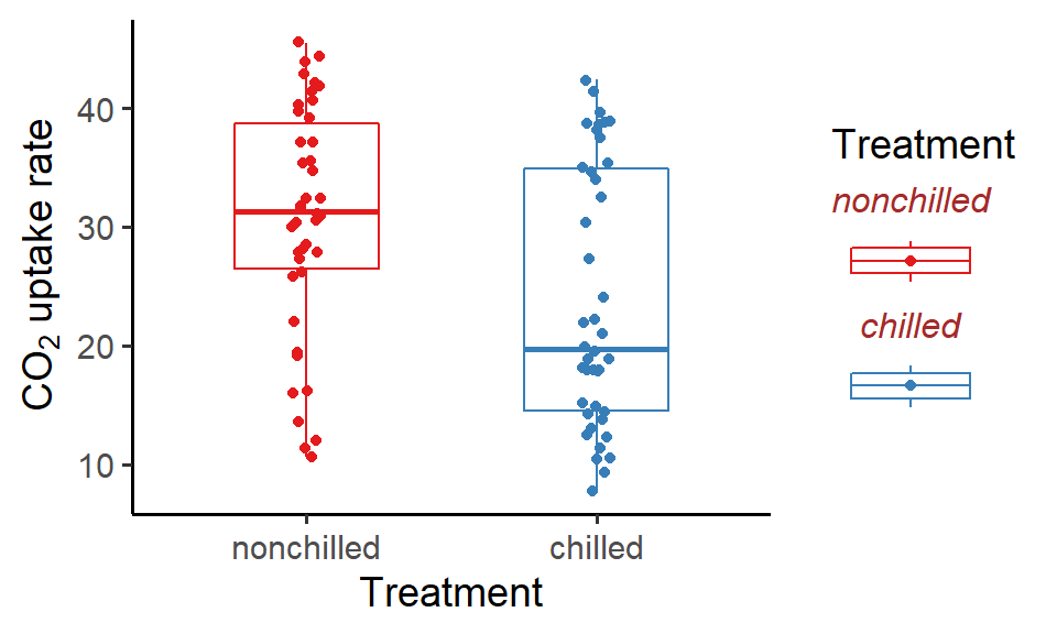
title.theme = element_text(size = 15, color = "darkgreen", face = "bold.italic"), # text appearance
title.hjust = 0.5, # horizontal alignment
title.vjust = 2)) # vertical alignment

(2) Legend labels
Similar to what we’ve done for the title, we can modify the position (relative to the legend keys) and text appearance of the labels as well as adjust the horizontal and vertical alignment. If we want to hide the labels, specify label = F.
P + guides(color = guide_legend(label = T,  # show the labels
                                label.position = "top",  # position
                                label.theme = element_text(size = 12, color = "brown", face = "italic"),  # text appearance
                                label.hjust = 0.5,  # horizontal alignment
                                label.vjust = 0.5))  # vertical alignment
(3) Legend keys
We can change the width and height of the legend keys. This is especially handy for adjusting the length (width) of line segments.
P + guides(color = guide_legend(keywidth = unit(0.25, "inches"),
                                keyheight = unit(0.5, "inches")))

(4) Legend layout
We can display the legend either horizontally or vertically, with legend items separated into several rows and columns. We can also reverse the order of the items.
P + guides(color = guide_legend(direction = "horizontal",  # direction of the legend
                                nrow = 1,  # number of rows
                                ncol = 2,  # number of columns
                                byrow = T,  # arrange the legend items row by row
                                reverse = T))  # reverse the legend items

(5) Change default mappings
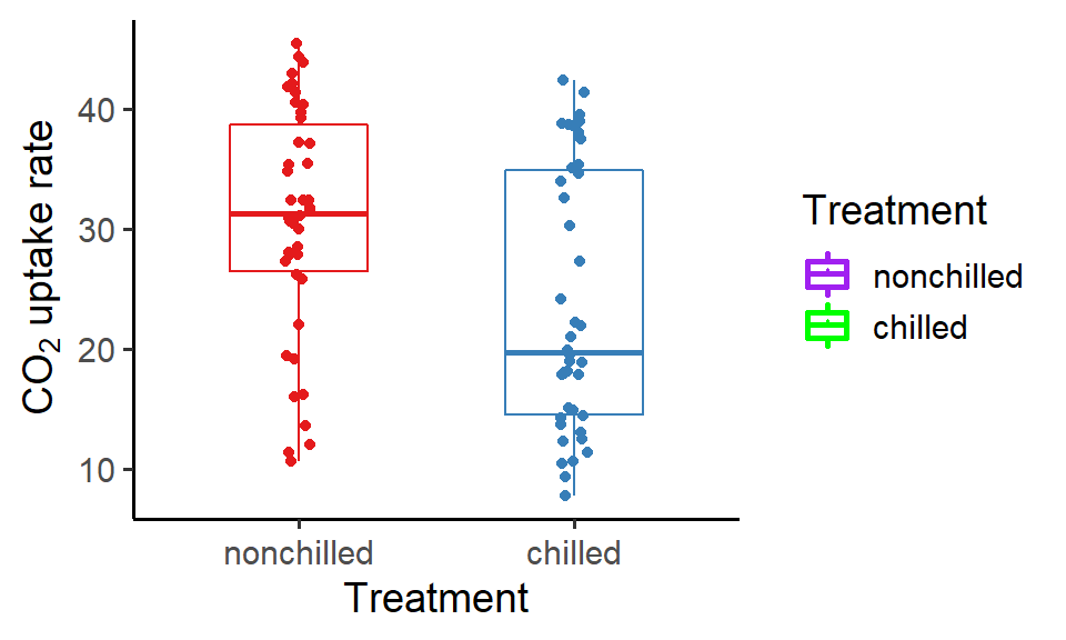
Suppose that we want to change the default aesthetic mappings, for example, the color of boxes, the shape of the points, and the size of the legend keys. We can do this by passing a list of new aesthetics to the argument override.aes:
P + guides(color = guide_legend(override.aes = list(color = c("purple", "green"),
                                                    shape = 17,
                                                    size = 1)))
(6) Multiple legends
Recall that the plant individuals come from two sites Quebec and Mississippi (variable “Type” in the dataset). We can map it to the “shape” aesthetic:
### Different shapes for the two sites
P_multi_legend <- ggplot(data = CO2) +
  geom_boxplot(aes(x = Treatment, y = uptake, color = Treatment), width = 0.5) +
  geom_point(aes(x = Treatment, y = uptake, color = Treatment, shape = Type), position = position_jitter(width = 0.05)) +
  labs(x = "Treatment", y = expression(paste(CO[2], " uptake rate"))) +
  theme_classic(base_size = 14) +
  scale_color_brewer(palette = "Set1")

P_multi_legend
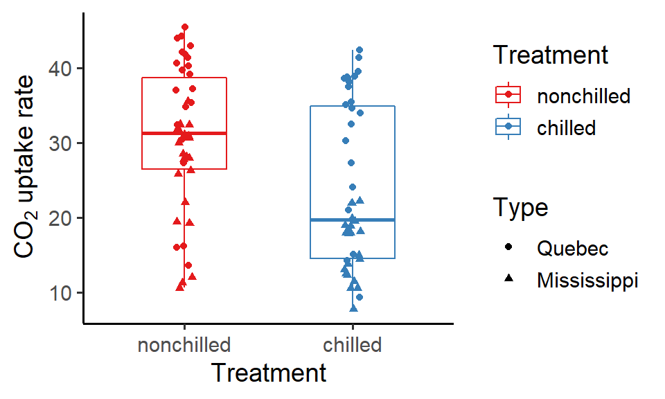
No we have two legends in the figure; time to make some changes for them!
Here, we apply guide_legend() individually to color and shape aesthetic and specify the respective arguments. Also, we use an additional argument order to tell ggplot the order in which the legends should be placed.
P_multi_legend + guides(color = guide_legend(title.position = "top",
                                             title.hjust = 0.5,
                                             label.position = "top",
                                             keywidth = unit(0.7, "inches"),
                                             keyheight = unit(0.8, "inches"),
                                             direction = "horizontal",
                                             order = 1),
                        shape = guide_legend(title = "Site",
                                             title.hjust = 0.5,
                                             label.position = "left",
                                             label.hjust = 0.5,
                                             label.vjsut = 0.5,
                                             keywidth = unit(0.5, "inches"),
                                             reverse = T,
                                             override.aes = list(size = 3),
                                             order = 2)
                        )
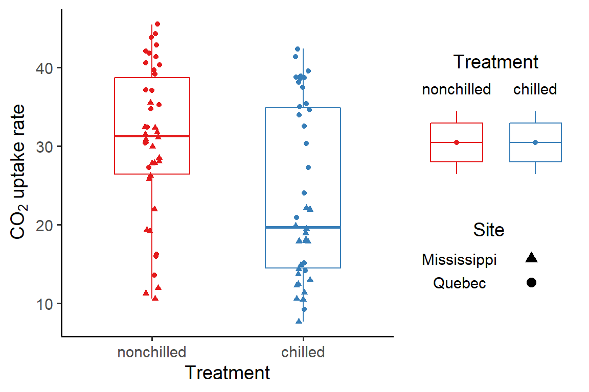
The changes don’t really make sense to me. Of course, it’s just a toy example showing the principles so that you can apply them next time to real-life situations.
Well that’s pretty much for now. But before we finish, it is worth mentioning that many of the arguments in guides() actually overlap with those in another legend function theme() (which will be the topic in another post of this series). So what’s the difference between these two functions? Which one should you use?
So the main difference is that, the arguments in guides() only affect the legends corresponding to the specified aesthetics, whereas the arguments in theme() will affect all the legends in the figure together. So if you have only one legend, using either function would give the same results. However, if you have multiple legends and you want to make different adjustments for each of them, then guides() is the go-to.
Summary
In this post, we’ve learned how to modify the appearance and layout of legend items in discrete ggplot legends using the function guides(). We can even customize the legend keys by overriding the default aesthetic mappings. Try playing around with the arguments a bit and I believe you will be able to make a nice legend(s) for your figure!
Hope you enjoy the reading and don’t forget to leave your comments and suggestions below if you have any!
