Week 4

Discrete exponential and logistic models

Lecture in a nutshell

• Discrete exponential growth (geometric growth):
  1. \(N_{t+1} = RN_{t}; N_{t+1} = R^{t}N_{0}\)
  2. Assumptions:
     • Closed population
     • Identical individuals
     • Unlimited resources: critical rates are constant
     • Discrete growth and census
  3. Pre-breeding census: \(N_{t+1} = (1 + \beta)(1-\delta) N_{t} = RN_{t}\)
  4. Cobweb plot: \(N_{t+1}\) vs. \(N_{t}\)
  5. Connection to the continuous model:\(N_{t+\Delta t} = (1+\beta \Delta t)(1-\delta \Delta t) N_{t}; \\\frac {dN}{dt} = \lim_{\Delta t \to 0} \frac {N(t+\Delta t)-N(t)}{\Delta t} = \lim_{\Delta t \to 0} (\beta N_{t}-\delta N_{t} - \beta \delta \Delta t) = (\beta-\delta)N_{t}\)
  6. Relationship between the intrinsic population growth rate r (which is a rate) and the finite rate of increase R (which is unitless): \(r = \frac {ln(R)}{h}\). \(h\) is the time interval between two population growth events. Note that R and cannot be directly manipulated; any math computations should be done on r (e.g., divide it by 10), and the modified r can later be converted back to R.

• Discrete logistic growth:
  1. \(N_{t+1} = N_{t} + rN_{t}(1-\frac {N_{t}}{K}) = N_{t}(1+r(1- \frac {N_{t}}{K})) = F_{(N_{t})}\)
  2. The equilibrium \(N^* = N_{t+1} = N_{t} \to N^* = 0, K\)
  3. Local stability analysis:
     • A small displacement from the equilibrium point at time \(t\): \(\epsilon_{t} = N_{t} - N^{*}\)
     • The behavior of this small displacement at next time step \(t+1\): \(\begin{aligned}\epsilon_{t+1}&=N_{t+1}-N^{*}\\&=F_{(N_{t+1})}-N^{*}\\&=F_{(N^{*}+\epsilon_{t})}-N^{*}\\&=F(N^*)+\epsilon_{t} \frac{dF}{dN}|_{N=N^*}+O_{(\epsilon_{t}^2)}-N^{*} \\&\approx \epsilon_{t}\frac{dF}{dN}|_{N = N^*}\\&=\lambda \epsilon\end{aligned}\)
  4. Stability criteria:
     • \(\lambda > 1\): unstable (smoothly moving away from the equilibrium)
     • \(0 < \lambda < 1\): stable (smoothly approaching the equilibrium)
     • \(-1 < \lambda < 0\): stable (damped oscillations converging towards the equilibrium)
     • \(\lambda < -1\): unstable (oscillations around the equilibrium)
  5. For the discrete logistic model:
     • \(N^{*} = 0\) is unstable (\(\lambda = 1+r > 1\))
     • \(K\) is stable only if \(0 < r < 2\) (\(\lambda = 1-r ~\&~ |\lambda| < 1\))

Lab demonstration

In this lab, we are going to model the discrete logistic population growth and visualize the system dynamics.

Part 1 - Model the discrete logistic population growth using for loops

library(tidyverse)

### (1) Set the parameters
r <- 1.8
K <- 500
N0 <- 10
time <- 100

### (2) Define the discrete logistic growth equation
log_fun <- function(r, N, K){N + r*N*(1-N/K)}  

### (3) Use for loop to iterate over the time sequence
pop_size <- numeric(time)
pop_size[1] <- N0

for (i in 2:time) {pop_size[i] <- log_fun(r = r, N = pop_size[i - 1], K = K)}

pop_data <- pop_size %>% 
  as.data.frame() %>% 
  rename(., pop_size = `.`) %>%
  mutate(time = 0:(time-1)) %>%
  relocate(time)

head(pop_data)

##   time  pop_size
## 1    0  10.00000
## 2    1  27.64000
## 3    2  74.64171
## 4    3 188.93980
## 5    4 400.51775
## 6    5 543.95762

Part 2. Visualize the population dynamics:

### Population trajectory
ggplot(pop_data, aes(x = time, y = pop_size)) + 
  geom_point() + 
  geom_line() +
  geom_hline(yintercept = K, color = "red", size = 1.2, linetype = "dashed") + 
  geom_text(x = time*1.02, y = K+50, label = "italic(K)", color = "red", size = 6.5, parse = T) +
  labs(y = expression(italic(N)), title = paste0("Discrete logistic growth", "\n", "(r = ", r, ", K = ", K, ", N0 = ", N0, ")")) + 
  scale_x_continuous(limits = c(0, time*1.05), expand = c(0, 0)) + 
  scale_y_continuous(limits = c(0, max(pop_size)*1.1), expand = c(0, 0)) + 
  theme_bw(base_size = 15) +
  theme(plot.title = element_text(hjust = 0.5))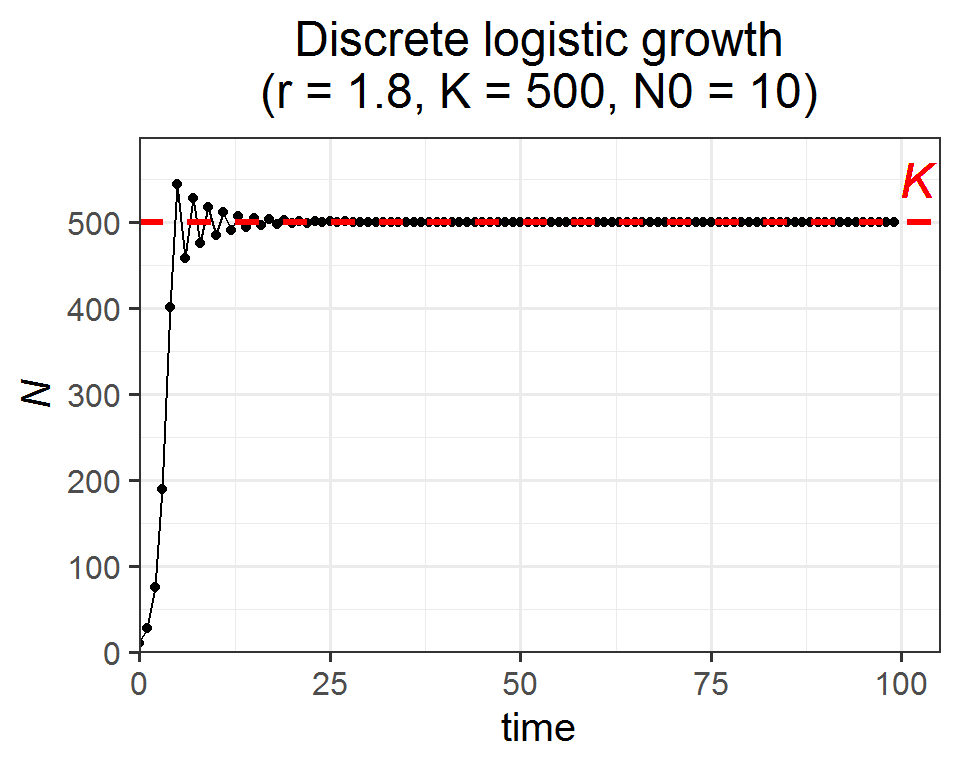

### Cobweb plot/logistic map
cobweb_data <- data.frame(Nt = rep(pop_size[-time], each = 2), 
                          Nt1 = c(0, rep(pop_size[-1], each = 2)[-length(rep(pop_size[-1], each = 2))]))

logistic_map <- data.frame(Nt = seq(0, (r+1)/r*K, by = 0.1)) %>%
  mutate(Nt1 = Nt + r*Nt*(1-Nt/K))

ggplot() + 
  geom_line(data = logistic_map, aes(x = Nt, y = Nt1), color = "green", size = 1.2) + 
  geom_path(data = cobweb_data, aes(x = Nt, y = Nt1), color = "blue", size = 0.5) + 
  geom_abline(slope = 1, intercept = 0, color = "red", size = 1) + 
  labs(x = expression(italic(N[t])),
       y = expression(italic(N[t+1])), 
       title = paste0("Cobweb plot/logistic map", "\n", "(r = ", r, ", K = ", K, ", N0 = ", N0, ")")) + 
  scale_x_continuous(limits = c(0, (r+1)/r*K*1.05), expand = c(0, 0)) + 
  scale_y_continuous(limits = c(0, max(pop_size)*1.1), expand = c(0, 0)) + 
  theme_bw(base_size = 15) +
  theme(plot.title = element_text(hjust = 0.5),
        panel.grid = element_blank())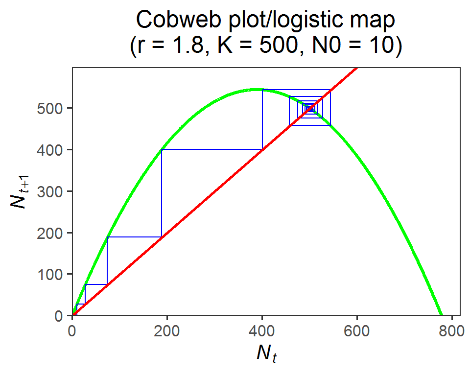

*The name “logistic map” comes from the fact that it maps the population size at one time step N_t to the value at the next time step N_t+1.

Here is a shiny app for the discrete logistic growth model. Feel free to play around with different inputs and see how the system dynamics change accordingly.

Additional readings

Simple mathematical models with very complicated dynamics

Assignments

Ricker Logistic Gowth Model

Suggested Solutions