Week 14
Disease dynamics and SIR models
Lecture in a nutshell
- Disease dynamics
- Compartmental models: assign individuals to different categories and model the transitions between them
- Density-based transmission vs. Frequency-based transmission: whether the rate of contacting other individuals scales with the population density. For example, in the SI model without demography,
- Density-based transmission: the growth of the infected individuals is \(\beta SI\)
- Frequency-based transmission: the growth of the infected individuals is \(\frac{\beta SI}{N}\)
- SI model without demography
- System of equations:
\(\begin{align}\frac {dS}{dt} =-\beta SI\end{align}\\\)\(\begin{align}\frac {dI}{dt} = \beta SI\end{align}\\\)
- The number of infected individuals will grow logistically and the disease will eventually infect the entire population.
- System of equations:
- SIR model without demography
- System of equations:
\(\begin{align}\frac {dS}{dt} =-\beta SI\end{align}\\\)\(\begin{align}\frac {dI}{dt} = \beta SI-\rho I\end{align}\\\)\(\begin{align}\frac {dR}{dt} = \rho I\end{align}\)
- \(R_{0}\): the number of secondary infections caused by one infected individual in a fully susceptible population (= per capita infection in a fully susceptible population*infectious time)
- For SIR model without demography, \(R_{0}\) is \(\frac{\beta}{\rho}S_{0}\)
- Can the disease spread at \(S_{0}\)? The invasion growth rate of I is \(\lim_{I \to 0} \frac{dI}{dt}\frac{1}{I} = \beta S_{0}-\rho\)
- If \(R_{0}\) > 1, IGR > 0, the disease will spread initially but later decline and eventually self-extinguish. Part of the population will be free from the infection. S and R coexist at the equilibrium.
- If \(R_{0}\) < 1, IGR < 0, disease cannot spread and will just gradually die out. The population will consist of mostly S and a few R at the equilibrium.
- System of equations:
- SIR model with demography
- System of equations:
\(\begin{align}\frac {dS}{dt} = \theta-\beta SI-\delta S\end{align}\\\)\(\begin{align}\frac {dI}{dt} = \beta SI-\rho I-\gamma I\end{align}\\\)\(\begin{align}\frac {dR}{dt} = \rho I-\delta R\end{align}\)
- \(R_{0}\) is \(\frac {\beta}{\rho+\gamma}\frac{\theta}{\delta}\)
- The equilibrium points \((S^{*}, I^{*}, R^{*})\):
- \(E_{DF}\) (disease-free equilibrium) = \((\frac{\theta}{\delta}, 0, 0)\)
- \(E_{E}\) (endemic equilibrium) = \((\frac{\gamma + \rho}{\beta}, \frac{\theta \beta-\delta(\gamma+\rho)}{\beta(\gamma+\rho)}, (\frac {\beta}{\rho+\gamma}\frac{\theta}{\delta}-1)\frac{\rho}{\beta})\) = \((\frac{1}{R_{0}}\frac{\theta}{\delta}, (R_{0}-1)\frac{\delta}{\beta}, (R_{0}-1)\frac{\rho}{\beta})\)
- Invasion analysis: \(\lim_{I \to 0} \frac{dI}{dt}\frac{1}{I} = \beta S_{DF}-\rho - \gamma\); disease can spread if \(\beta \frac{\theta}{\delta} -\rho - \gamma > 0\) (or \(R_{0} > 1\))
- Local stability analysis:
- \(E_{DF}\)
- \(J_{DF} = \begin{vmatrix} -\delta & -\beta S^{*} & 0\\0 & \beta S^{*}-\rho-\gamma & 0\\0 & \rho & -\delta\end{vmatrix}\)
- Eigenvalues: \(-\delta\), \(-\delta\), \(\beta S^{*}-\rho-\gamma\)
- Locally stable if \(\beta S^{*}-\rho-\gamma < 0\), that is, \(R_{0} < 1\)
- \(E_{E}\)
- \(J_{E} = \begin{vmatrix} -\beta I^{*}-\delta & -\beta S^{*} & 0\\\beta I^{*} & 0 & 0\\0 & \rho & -\delta\end{vmatrix}\)
- Characteristic equation: \((\delta + \lambda)(\lambda^{2}+(\beta I^{*}+\delta)\lambda+\beta^{2}I^{*}S^{*}) = 0\)
- Locally stable if \(I^{*} > 0\) (\(I^{*}\) is feasible), that is, \(R_{0} > 1\)
- \(J_{E} = \begin{vmatrix} -\beta I^{*}-\delta & -\beta S^{*} & 0\\\beta I^{*} & 0 & 0\\0 & \rho & -\delta\end{vmatrix}\)
- \(E_{DF}\)
- System of equations:
Lab demonstration
In today’s lab, we are going to simulate the SIR model with demography and visualize two types of disease dynamics: (1) the endemic equilibrium, at which the S, I, and R all coexist, and (2) the disease-free equilibrium, at which the disease will die off and only S remains.
\(\begin{align}\frac {dS}{dt} = \theta-\beta SI-\delta S\end{align}\\\)
\(\begin{align}\frac {dI}{dt} = \beta SI-\rho I-\gamma I\end{align}\\\)
\(\begin{align}\frac {dR}{dt} = \rho I-\delta R\end{align}\)
library(tidyverse)
library(deSolve)

SIR_model_fun <- function(theta, beta, delta, rho, gamma, title){

  # model specification
  SIR_model <- function(times, state, parms) {
    with(as.list(c(state, parms)), {
      dS_dt = theta - beta*S*I - delta*S
      dI_dt = beta*S*I - rho*I - gamma*I
      dR_dt = rho*I - delta*R
      return(list(c(dS_dt, dI_dt, dR_dt)))
    })
  }

  # model parameters
  times <- seq(0, 1000, by = 1)
  state <- c(S = 25, I = 0.1, R = 0)
  parms <- c(theta = theta, beta = beta, delta = delta, rho = rho, gamma = gamma)

  # model application
  SIR_out <- ode(func = SIR_model, times = times, y = state, parms = parms)

  # visualization
  SIR_out %>%
    as.data.frame() %>%
    pivot_longer(cols = -time, names_to = "state", values_to = "N") %>%
    mutate(state = fct_relevel(state, "S", "I", "R")) %>%
    ggplot(aes(x = time, y = N, color = state)) +
    geom_line(size = 1.5) +
    theme_classic(base_size = 14) +
    labs(x = "Time", y = "N", title = title) +
    scale_x_continuous(limits = c(0, 1010), expand = c(0, 0)) +
    scale_y_continuous(limits = c(0, 55), expand = c(0, 0)) +
    scale_color_brewer(name = NULL, palette = "Set1") +
    theme(plot.title = element_text(hjust = 0.5))

}
### Epidemic equilibrium
SIR_model_fun(theta = 0.25, beta = 0.01, delta = 0.01, rho = 0.02, gamma = 0.02, title = "Epidemic equilibrium")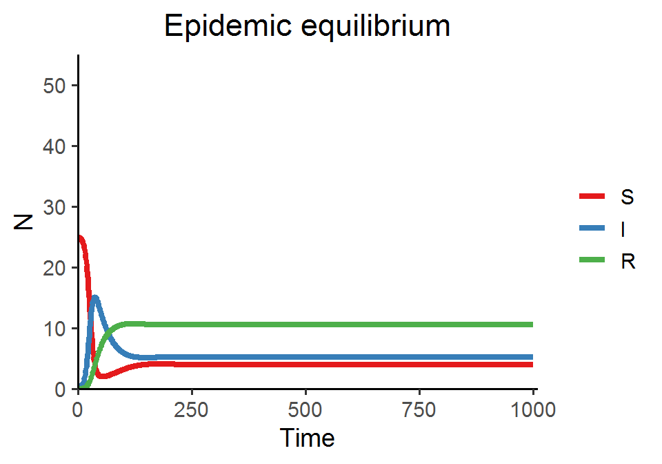
### Disease-free equilibrium
SIR_model_fun(theta = 0.25, beta = 0.01, delta = 0.01, rho = 0.3, gamma = 0.02, title = "Disease-free equilibrium")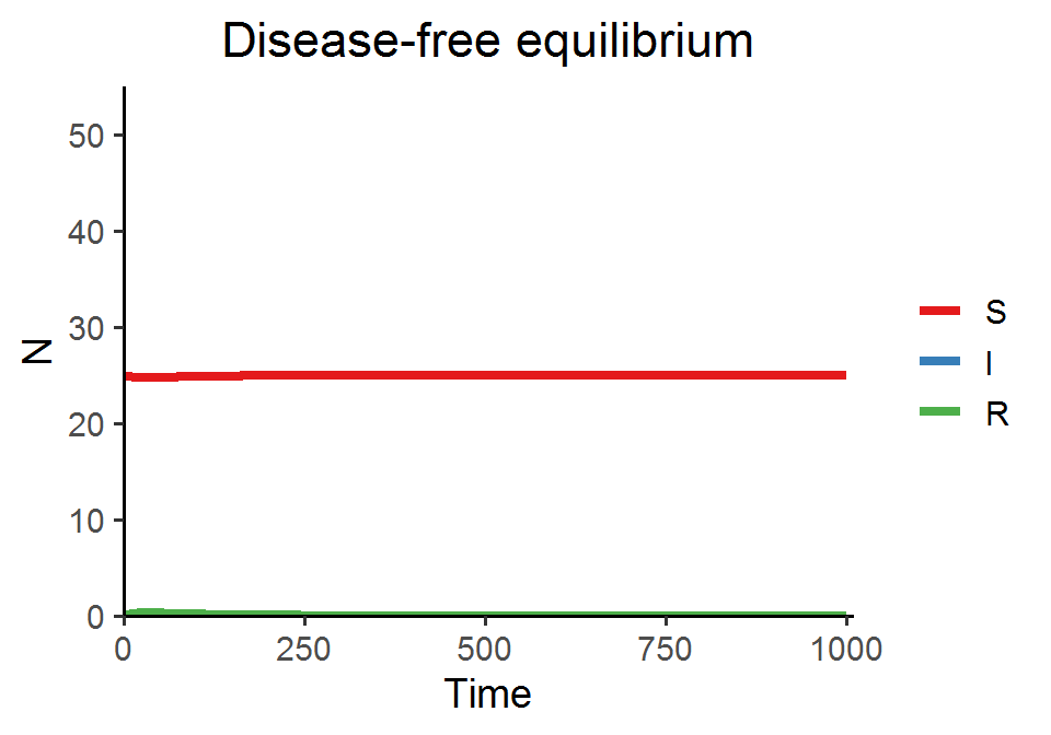
By increasing the recovery rate \(\rho\) in the second example, we drive the basic reproduction number \(R_{0}\) below 1, and thus the disease will not spread and the system reaches the disease-free equilibrium.