Week 3
Lecture in a nutshell
- Model derivation:
- Population growth rate: \(Birth - Death + Immigration - Emigration\)
- Per capita growth rate: \((birth - death + immigration - emigration)\times N\).
- Assumptions:
- Closed population: \(Immigration\) = \(Emigration = 0\)
- All individuals are identical: no genetic/age/stage structure
- Continuous population growth without time lag
- Per capita birth and death rates are time-independent BUT density-dependent
- Resource is limited: negative density-dependence (NDD) \(\frac{dr_{(N)}}{dt} < 0\)
- Linear density-dependence: \(b_{(n)} = b_{0}-b_{N}N\); \(d_{(n)} = d_{0}+d_{N}N\) \(\begin{aligned}\frac{dN}{dt}&=(b_{0}-b_{N}N-d_{0}-d_{N}N)N\\&=((b_{0}-d_{0})-(d_{N}+b_{N})N)N\\&=(r_{0}-\alpha N)N\\&=r_{0}N(1-\frac{N}{K})\end{aligned}\)
- Integration of the differential equation
- \(N_{(t)} = \frac{K}{1-\frac{N_{0}-K}{N_{0}}e^{-r_{0}t}}\)
- Equilibrium \(N^*\): good candidates where the system will end up
- \(\frac{dN}{dt} = f_{(N^*)} = r_{0}N^{*}(1-\frac{N^*}{K}) = 0\); \(N^* = 0, K\)
- Attracting (Stable) vs. Repelling (Unstable) vs. Saddle
- Graphical analysis
- Plot the function \(\frac{dN}{dt} = f(N)\) and determine the direction of change (positive/negative) on both sides of the equilibrium points \(N^*\)
- Local stability analysis
- A small “displacement” from the equilibrium: \(\epsilon_{(t)} = N - N^*\)
- Examine how \(\epsilon_{(t)}\) changes over time (i.e., the behavior of the small displacement): \(\frac{d\epsilon_{(t)}}{dt} = f(N-N^*) = f(N^*) + \epsilon \frac{dN}{dt}|_{N = N^*} + O_{(\epsilon^2)} \approx \epsilon\frac{dN}{dt}|_{N = N^*} = \lambda \epsilon\); \(\epsilon_{(t)} = \epsilon_{0}e^{\lambda t}\)
(the behavior of \(\epsilon_{(t)}\) is determined by the sign of \(\lambda\)) - General procedure: take derivative of the differential equation with respect to \(N\) and evaluate it at the equilibrium point \(N^*\):
- \(\frac{dN}{dt}|_{N = N^*} = \lambda > 0\): unstable equilibrium
- \(\frac{dN}{dt}|_{N = N^*} = \lambda < 0\): stable equilibrium
Lab demonstration
In this lab, we will solve the differential equation for logistic population growth and visualize how the population sizes change over time. Have a quick review of the lab section in Week 2.
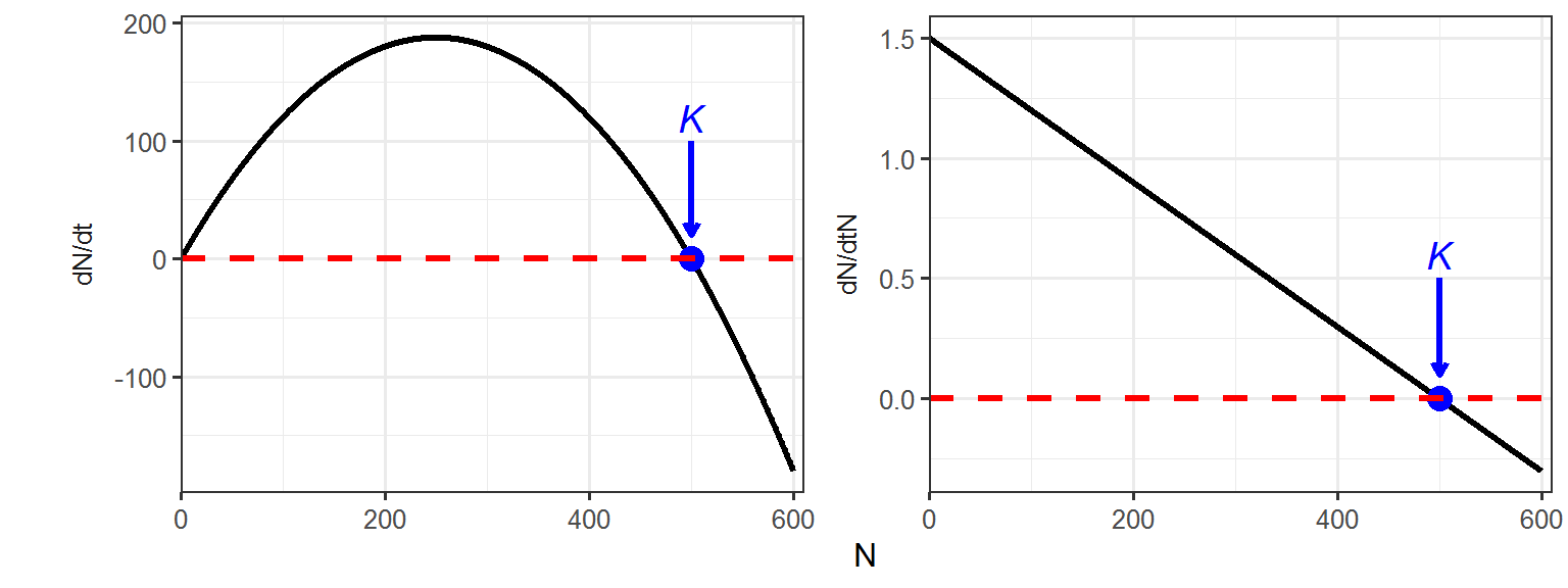
We will also take a look at how population growth rate (\(\frac{dN}{dt}\)) and per capita growth rate (\(\frac{dN}{dtN}\)) change with population size (\(N\)).
Part 1 - Solving the logistic growth equation and visualize the results
library(tidyverse)
library(deSolve)

### Model specification
logistic_model <- function(times, state, parms) {
  with(as.list(c(state, parms)), {
    dN_dt = r*N*(K-N)/K  # logistic growth equation
    return(list(c(dN_dt)))  # return the results
  })
}

### Model application
times <- seq(0, 10, by = 0.1)  # time steps to integrate over
state <- c(N = 10)  # initial population size
parms <- c(r = 1.5, K = 500)  # intrinsic growth rate and carrying capacity

# run the ode solver
pop_size <- ode(func = logistic_model, times = times, y = state, parms = parms)

### Visualize the results
ggplot(data = as.data.frame(pop_size), aes(x = time, y = N)) +
  geom_point() +
  labs(title = paste0("Logistic Growth \n (r = ", parms["r"], ", K = ", parms["K"], ")")) +
  theme_classic(base_size = 12) +
  theme(plot.title = element_text(hjust = 0.5)) +
  scale_x_continuous(limits = c(0, 10.5), expand = c(0, 0)) +
  scale_y_continuous(limits = c(0, max(as.data.frame(pop_size)$N)*1.1), expand = c(0, 0))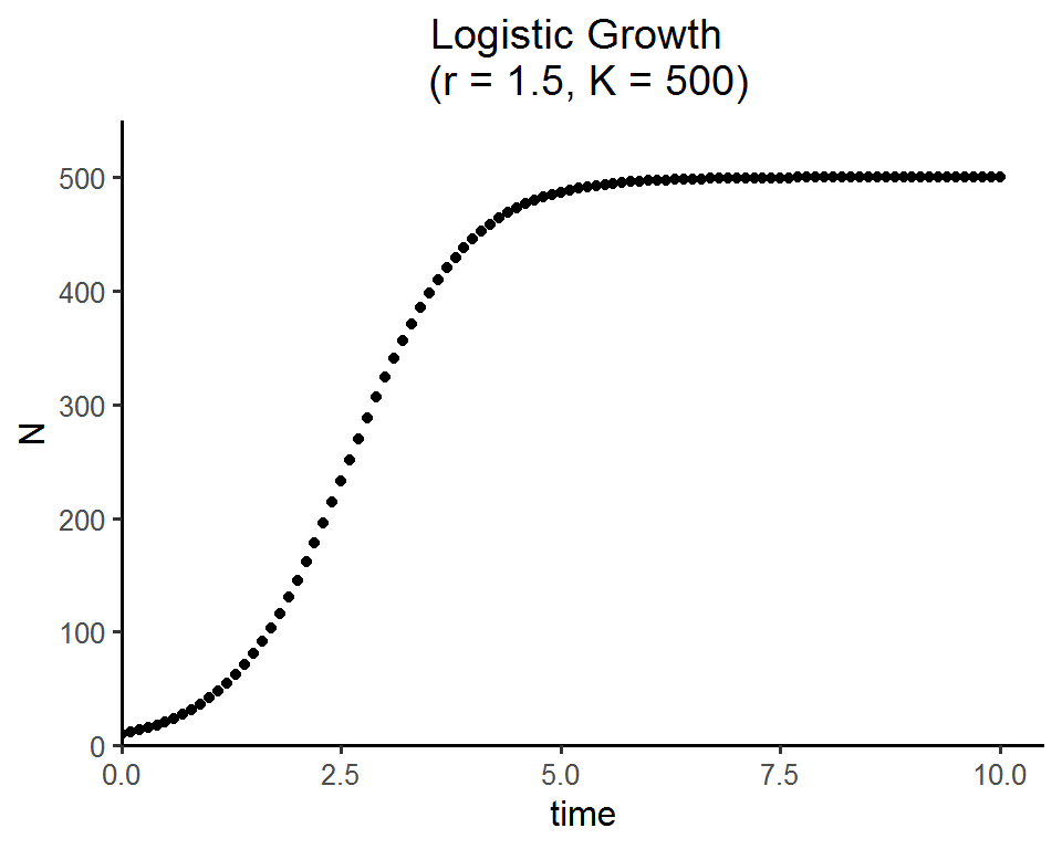
Here is an interactive web app for the logistic growth model. Feel free to play around with the parameters/values and see how the population trajectories change. Please select a set of parameters of your choice and reproduce the output figure you see in this app.
Part 2 - The relationship between population growth rate (\(\frac{dN}{dt}\))/per capita growth rate (\(\frac{dN}{dtN}\)) and population size (\(N\))
# parameters
r <- 1.5
K <- 500

# a vector of population sizes
N <- 0:600

# calculate the population growth rates and per capita growth rates
dN_dt <- r*N*(K-N)/K
dN_dtN <- r*(K-N)/K

# organize into a dataframe
logistic_data <- data.frame(N, dN_dt, dN_dtN) %>%
  pivot_longer(cols = c(dN_dt, dN_dtN),
               names_to = "vars",
               values_to = "values")

# plot
K_df <- data.frame(xend = c(500, 500),
                   yend = c(20, 0.1),
                   xstart = c(500, 500),
                   ystart = c(100, 0.5),
                   labels = c("italic(K)", "italic(K)"),
                   vars = c("dN_dt", "dN_dtN"))

ggplot(data = logistic_data, aes(x = N, y = values)) +
  geom_line(size = 1.2) +
  geom_point(x = 500, y = 0, size = 4, color = "blue") +
  geom_hline(yintercept = 0, linetype = "dashed", color = "red", size = 1.2) +
  labs(x = "N", y = "") +
  facet_wrap(~vars,
             ncol = 2,
             scales = "free_y",
             strip.position = "left",
             labeller = as_labeller(c(dN_dt = "dN/dt",
                                      dN_dtN = "dN/dtN"))) +
  theme_bw(base_size = 12) +
  theme(strip.background = element_blank(),
        strip.placement = "outside",
        legend.position = "top",
        legend.title = element_blank()) +
  scale_x_continuous(limits = c(0, 610), expand = c(0, 0)) +
  geom_segment(data = K_df,
               aes(x = xstart, y = ystart, xend = xend, yend = yend),
               arrow = arrow(length = unit(0.03, "npc")),
               size = 1.2,
               color = "blue") +
  geom_text(data = K_df,
            aes(x = xstart, y = ystart*1.2, label = labels),
            size = 5,
            color = "blue",
            parse = T)