Introduction
Google Maps is arguably the most commonly used online map application in our everyday life: for navigation, for finding specific places, for measuring the distance, just to name a few. We also use Google Maps frequently in presentations, for example, showing a satellite image and the location of the study sites. Traditionally, what we’ll do is going to the Google Maps webpage, taking a screen shot of the map, cropping and editing it in PowerPoint.
Now, thanks to the extension package ggmap, we can get rid of the tedious work and directly retrieve Google Maps tiles from R and plot them in ggplots. We can then add polygons, lines, and points to the maps. This is exactly the goal of this post, and I’m going to show you how to do these things. The post will be short but handy!
Create maps using Google Maps tiles
Before we start, there is one thing you need to do: registering with Google and setting up an API key for the map platform. This is required to retrieve data from Google Map. Visit this page for how to do this.
After you get your API key, paste it into the function register_google() and you’re all set:
library(ggmap)
register_google(key = "your key")
Get the map tiles
The first step is to get the map tiles of the desired area using the function get_googlemap(). There are two ways to do so:
- By location: supply the name of the place (e.g., “New York City”)
- By longitude and latitude: supply the lon-lat coordinates of the place
The place will occur at the center of the map. To control the extent of the map area, you can specify an additional argument “zoom”, which ranges from 3 to 21. As a rule of thumb, 3 gives continent-level view, 12 gives city-level view, and 21 gives building-level view. Experiment the values a bit to get the desired outcome.
library(tidyverse)

### Get the map data
my_location <- "Ithaca"  # location
my_lon_lat <- c(-76.50, 42.44)  # lon-lat pair

my_location_map <- get_googlemap(my_location, zoom = 12)
my_lon_lat <- get_googlemap(my_lon_lat, zoom = 12)
There is a useful helper function geocode() that can find the longitude and latitude coordinates of a given location:
### Find the lon-lat coordinates of the given location
geocode("Ithaca")
# A tibble: 1 × 2
lon lat
<dbl> <dbl>
1 -76.5 42.4Draw the map
After we get the map tiles of the area, it’s time to draw the map! Super simple: just pass the map tiles to ggmap():
map_by_location <- ggmap(my_location_map) +
  labs(title = "By location") +
  theme(plot.title = element_text(hjust = 0.5))

map_by_lon_lat <- ggmap(my_lon_lat) +
  labs(title = "By lon-lat pair") +
    theme(plot.title = element_text(hjust = 0.5))

library(patchwork)
map_by_location + map_by_lon_lat
Let’s also try out different zoom values:
### Different zoom values
my_maps_zooms <- lapply(c(3, 6, 10, 13, 17, 21), function(x){
  get_googlemap(my_location, zoom = x) %>%
    ggmap() +
    labs(title = paste0("zoom = ", x)) +
    theme(plot.title = element_text(hjust = 0.5))
})

patchwork::wrap_plots(my_maps_zooms, ncol = 3, nrow = 2, byrow = T)
Besides the default terrain map, we can also get the road map, satellite image, or a hybrid of them:
### Different map types
my_maps <- lapply(c("terrain", "roadmap", "satellite", "hybrid"), function(x){
  get_googlemap(my_location, zoom = 12, maptype = x) %>%
    ggmap() +
    labs(title = x) +
    theme(plot.title = element_text(hjust = 0.5))
})

patchwork::wrap_plots(my_maps, ncol = 2, nrow = 2, byrow = T)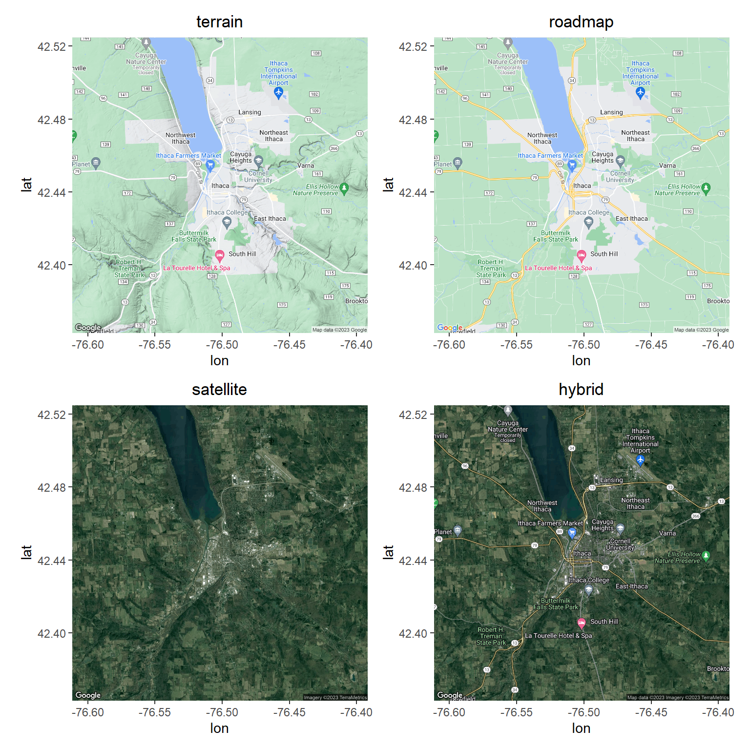
Add a polygon and points to a satellite image
We can spice up the “plain” map by adding polygons/lines/points to it. Here, I’m going to draw the boundary of Ithaca City and show the locations of the city street trees on a Google satellite image. The data (shapefiles) can be download from City of Ithaca Community Data Portal.
We’ll first retrieve the zip files from the GitHub repository, unzip them, and read in the shapefiles using the function st_read() from the package sf (see my previous post on making maps with sf!). Next, we can add the shapefile data to the satellite image using geom_sf(). Note that we need to set “inherit.aes = F” so that geom_sf() will not use the aesthetics from the global plot that are used for the satellite image.
Let’s take a look at how it works:
### Download the zip files from the GitHub repository and unzip them
# (1) city boundary
url_city_boundary <- "https://github.com/GenChangHSU/ggGallery/blob/master/_posts/2023-10-26-post-30-ggplot-map-series-no4-creating-maps-with-ggmap/Municipal_Boundary.zip?raw=TRUE"
download.file(url_city_boundary, "Municipal_Boundary.zip", mode = "wb")
unzip("Municipal_Boundary.zip")

# (2) city trees
url_city_trees <- "https://github.com/GenChangHSU/ggGallery/blob/master/_posts/2023-10-26-post-30-ggplot-map-series-no4-creating-maps-with-ggmap/City_Managed_Trees.zip?raw=TRUE"
download.file(url_city_trees, "City_Managed_Trees.zip", mode = "wb")
unzip("City_Managed_Trees.zip")

### Read in the shapefiles of city boundary and city trees
library(sf)

city_boundary <- st_read("./Municipal_Boundary/Municipal_Boundary.shp", quiet = T)
city_trees <- st_read("./City_Managed_Trees/City_Managed_Trees.shp", quiet = T)

### Add the city boundary and city trees to a satellite image
get_googlemap(my_location, zoom = 13, maptype = "satellite") %>%
  ggmap() +
  geom_sf(data = city_boundary, fill = NA, color = "red", linewidth = 1, inherit.aes = F) +  # need to set "inherit.aes = F"
  geom_sf(data = city_trees, color = "forestgreen", size = 0.1, inherit.aes = F)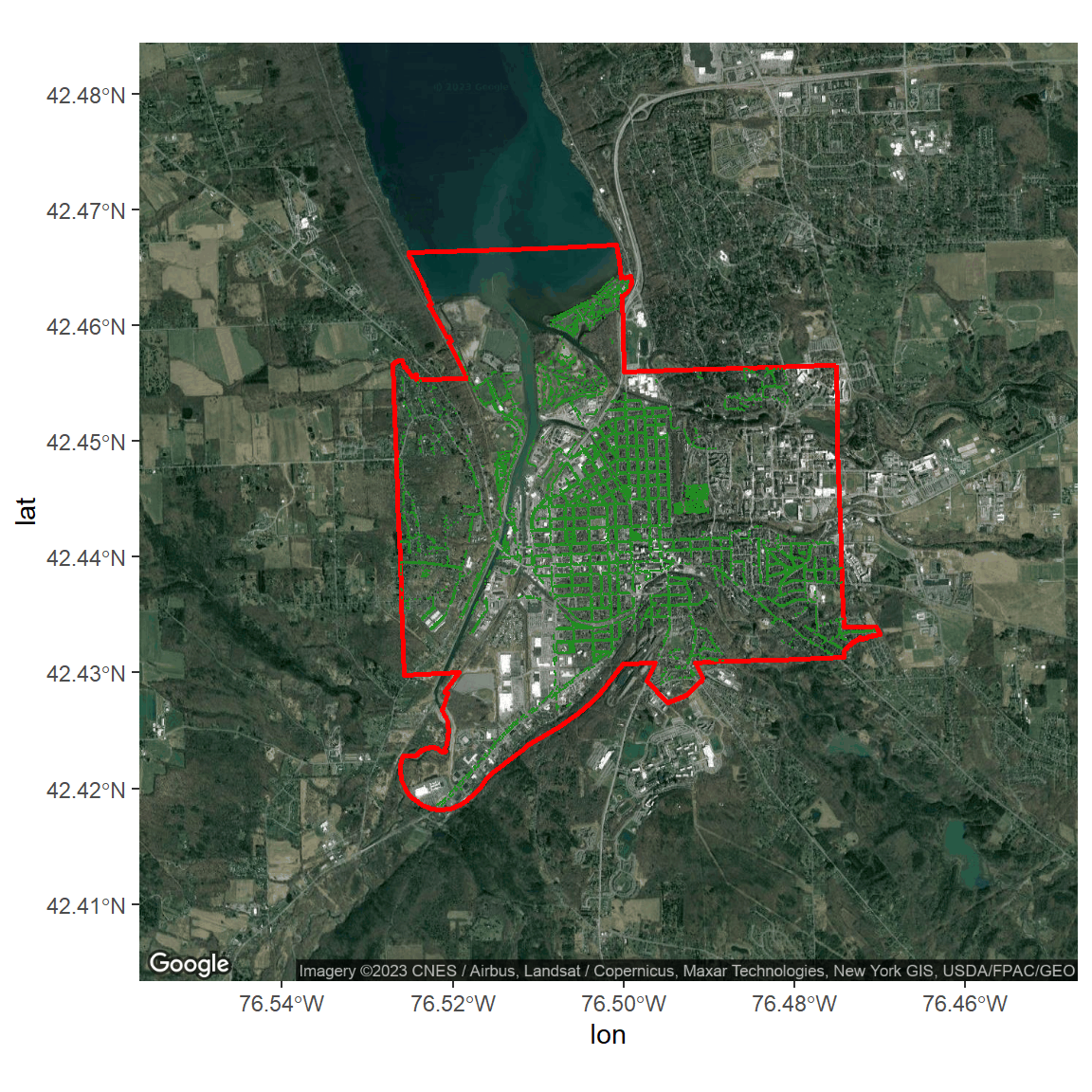
Voila!
Summary
In this post, we learned how to create maps using Google Maps tiles with the package ggmap. First, we got the map tiles of the area of interest using get_googlemap(), and then we passed the data to ggmap() to draw the map. We also tried out a few different zoom values and map types. Finally, we polished a Google satellite image by adding a polygon and points to it. Next time, you can use this method to create a map to show your study site/plot and the locations of the species/organisms!
Hope you learn something useful from this post and don’t forget to leave your comments and suggestions below if you have any!
