Introduction
OpenStreetMap (OSM) is a free open global geographic database maintained by a community of volunteers and contributors. The map data in OSM contain almost every physical feature on the ground, from natural properties like mountain peaks, water bodies, and vegetation types, to human-made structures like roads, shops, and trails (see this website for a complete list of the map features). These data are used by a great number of websites and software apps for their maps.
In this post, we’re going to visualize the rivers in Taiwan in ggplots using data in OSM. Hopefully, after reading the post, you will be able to make good use of this database to make your own awesome ggplot maps!
Create the map
Let’s jump right in! First, we’ll obtain the river data of Taiwan from OSM, and then we’ll visualize them in ggplots. Finally, we’ll have some fun with the map by making it artistic.
(1) Prepare the data
The package osmdata allows users to download map data from OSM for any given area. This involves three steps:
Defining a bounding box using the function
opq(bbox = ). The argument “bbox” can be either a character string of the location name (e.g.,"Taipei"), or four numerical values specifying the minimal and maximal longitudes and latitudes of the area (e.g.,c(120, 20, 120.5, 21)).Building an osmdata query using the function
add_osm_feature(key = , value = ). The requested data are specified using “key-value” pairs, with key representing the major category of the data and the value representing the more specific feature type under that major category. Take a look at the website for the available features.Retrieving OSM data with the query. The function
osmdata_sf()will send the query to OSM, obtain the requested data, and return them in the “simple feature (sf)” format.
Let’s see a worked example below: We got a vector of the county names in Taiwan and looped over the vector to retrieve the OSM data for each county. Because the river information is stored as a list of simple feature lines in the returned object, we further extracted it for each county and merged all the lists into a single dataframe.
library(tidyverse)
library(osmdata)

### Get the county names in Taiwan
# library(remotes)
# install_github("wmgeolab/rgeoboundaries")  # install the package if you haven't
library(rgeoboundaries)  # for the function "geoboundaries()"
Taiwan_county_names <- geoboundaries("Taiwan", "adm1") %>%
  as.tibble() %>%
  filter(!shapeName %in% c("Kinmen", "Matsu Islands")) %>%  # exclude Kinmen and Matsu islands for better visualization
  pull(shapeName)

### Obtain the OSM river data for each county
Taiwan_river_osmdata <- Taiwan_county_names %>%
  map(., ~ opq(bbox = .x, timeout = 100) %>%  # need to increase the "timeout" (default to 25 seconds) for larger queries
        add_osm_feature(key = 'waterway', value = "river") %>%
        osmdata_sf()) %>%
  `names<-`(Taiwan_county_names)

### Extract the list of simple feature lines for each county and merge them into a single dataframe
Taiwan_river_osmdata_lines <- Taiwan_river_osmdata %>%
  map(., ~ .x$osm_lines) %>%
  bind_rows(.id = "county")

### Take a look at the dataframe
Taiwan_river_osmdata_lines %>%
  select(osm_id, county, geometry) %>%
  head()
Simple feature collection with 6 features and 2 fields
Geometry type: LINESTRING
Dimension: XY
Bounding box: xmin: 120.9303 ymin: 24.65206 xmax: 121.5074 ymax: 25.17773
Geodetic CRS: WGS 84
osm_id county geometry
25887259...1 25887259 Hsinchu County LINESTRING (121.4859 25.042...
27696480...2 27696480 Hsinchu County LINESTRING (121.23 24.89155...
27696492...3 27696492 Hsinchu County LINESTRING (121.1948 24.888...
91846587...4 91846587 Hsinchu County LINESTRING (121.0272 24.844...
91846590...5 91846590 Hsinchu County LINESTRING (121.1085 24.730...
91907207...6 91907207 Hsinchu County LINESTRING (121.2379 24.652...Create the river map
Now we have the river data on hand, we can visualize them in ggplots! The river data is an “sf” object, which can be passed directly to the function geom_sf() for plotting (also see my previous post on making simple feature maps in ggplots!). We’ll also draw the boundary of Taiwan as the base map.
### Taiwan boundary data
Taiwan_boundary_adm0 <- geoboundaries("Taiwan", "adm0")

### The river map of Taiwan
ggplot() +
  geom_sf(data = Taiwan_boundary_adm0, fill = "grey90", alpha = 0.7) +
  geom_sf(data = Taiwan_river_osmdata_lines, linewidth = 0.1, color = "steelblue") +
  coord_sf(xlim = c(119, 123), ylim = c(21.7, 25.5)) +
  theme_minimal() +
  theme(panel.background = element_rect(color = "black"),
        panel.grid.major = element_blank())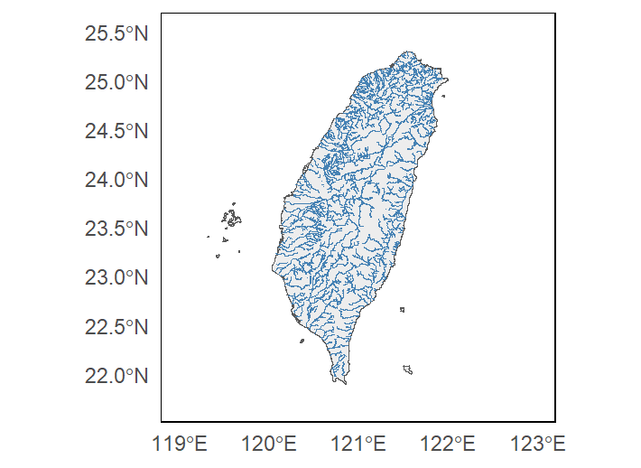
Here we go!
Make it artistic
Let’s modify the appearance of the map to make it artistic:
ggplot() +
  geom_sf(data = Taiwan_river_osmdata_lines, aes(color = county), linewidth = 0.1, show.legend = F) +
  coord_sf(xlim = c(119, 122.5), ylim = c(21.7, 25.5)) +
  theme_void() +
  theme(panel.background = element_rect(fill = "black"))
The veins of Taiwan clear at a glance!
Summary
To summarize what we did, we obtained the river data of Taiwan from OSM using the package osmdata and visualized them in ggplots. I showcased the river data here, but the same principle applies to other features as well, and you can take advantage of them to create great thematic maps.
Hope you learn something useful from this post and don’t forget to leave your comments and suggestions below if you have any!
