Introduction
The ggplot2 package, one of the most popular packages in R, is a powerful tool for making elegant data visualizations based on the grammar of graphics. Recently, the gt package, the ggplots for tables, came on the scene. Based on the grammar of tables, it makes creating tables in R much more convenient and versatile.
The main idea of gt is to build tables from a set of components such as the header, the stub, the column labels, the body, and the footer. We can compose each of these parts individually, customize their formats and styles, and finally put them together. gt is itself an amazing package for awesome table displays. But what’s even more exciting is that it can be used in conjunction with ggplots, which will certainly enhance the effectiveness of data visualizations and I can’t wait to try it out.
To this end, I’ll do a small data viz project in this post to visualize the top ten bird-window collision species in Taiwan. Bird-window collisions, quite literally, are birds colliding with windows of buildings or other human-made structures. Study 1 has shown that this is one of the leading anthropogenic bird mortality sources, killing hundreds of millions of birds each year.
At the end of the post, you’ll find out what the top ten bird-window collision species in Taiwan are. Also, this post is not just a data viz practice; hopefully, it can help raise the awareness of this concerning wildlife issue and make the invisible visible. Finally, a shout-out to my friend Chi-Heng Hsieh, who kindly provided the bird-window collision data for this post!
Let’s build the table
Before we start off, I would like to give you an overall idea of what the table will look like: It has a first column showing the images of the bird species, a second column showing the species names along with a short description of each, a third column showing the total number of collision cases for each species between 2010 and 2022, and a fourth column showing the annual collision trends for each species over this 13-year period.
In the following section, I’ll break down the process into several steps so that it’s easier to follow and understand what the code is doing.
1. Data preparation and summary
As always, the first step in a data project is to prepare the data. After reading in the data set, we count the total number of collision cases between 2010 and 2022, as well as the number of species recorded in this period. Because there are some cases where the colliding individuals were only identified to the genus or family level, we filter them out before tallying the unique species names.
library(tidyverse)

### Read in the data set
bwc_data <- read_csv("https://raw.githubusercontent.com/GenChangHSU/ggGallery/master/_posts/2023-02-18-post-24-gt-and-ggplot-visualizing-bwc-in-taiwan/BWC_data.csv")

### Total cases between 2010 and 2022
bwc_data %>%
  filter(year >= 2010) %>%
  nrow()
[1] 3608### Number of collision species
bwc_data %>%
filter(year >= 2010) %>%
rowwise() %>%
filter(length(unlist(str_split(species, " "))) == 2) %>% # remove the families
filter(!str_detect(species, "sp\\.")) %>% # remove the genera
distinct(species) %>%
nrow()[1] 1702. The top ten collision species
Next, we count the number of collision cases by species, select the top ten species, and add their common names.
bwc_top_collision_df <- bwc_data %>%
  filter(year >= 2010) %>%
  group_by(species) %>%
  summarise(n = n()) %>%
  arrange(desc(n)) %>%
  slice_head(n = 10) %>%
  mutate(common_name = c("Taiwan barbet",
                         "Asian emerald dove",
                         "Spotted dove",
                         "Eurasian tree sparrow",
                         "Crested goshawk",
                         "Common kingfisher",
                         "Light-vented bulbul",
                         "Pale thrush",
                         "Swinhoe's white-eye",
                         "Oriental turtle dove"))
3. The images and short descriptions of the species
Now, we get the images of the top ten collision species from the The Cornell Lab of Ornithology’s Macaulay Library and add a short description of each species based on the information on eBird. The descriptions are wrapped inside the HTML <tags> to customize the text appearance. (You’ll see how this works later.)
### The species images
bwc_top_collision_df <- bwc_top_collision_df %>%
  mutate(image = c("https://cdn.download.ams.birds.cornell.edu/api/v1/asset/85866641/480",
                   "https://cdn.download.ams.birds.cornell.edu/api/v1/asset/65752231/320",
                   "https://cdn.download.ams.birds.cornell.edu/api/v1/asset/351501301/480",
                   "https://cdn.download.ams.birds.cornell.edu/api/v1/asset/391684791/320",
                   "https://cdn.download.ams.birds.cornell.edu/api/v1/asset/352462361/320",
                   "https://cdn.download.ams.birds.cornell.edu/api/v1/asset/387920071/320",
                   "https://cdn.download.ams.birds.cornell.edu/api/v1/asset/147572491/320",
                   "https://cdn.download.ams.birds.cornell.edu/api/v1/asset/465299711/480",
                   "https://cdn.download.ams.birds.cornell.edu/api/v1/asset/299650741/480",
                   "https://cdn.download.ams.birds.cornell.edu/api/v1/asset/472227361/480"))

### Short descriptions of the species
library(glue)

bwc_top_collision_df <- bwc_top_collision_df %>%
  mutate(description = c(
  "Distinctive <span style = 'color: green'>endemic</span> with a bright green body and a head in red, blue, yellow,
  and black. Vocalization characterized by a frog-like croaking.",
  "Brightly-colored dove of the forest floor with emerald green wings, coral-red bill, and ash-gray forehead.
  Male with an extensive silver cap.",
  "Tame dove commonly found in open forests, fields, and parks.
  Brown overall with a rosy breast and a unique white-spotted black nape patch.",
  "Frequent visitor of urban areas and human settlements. Easily identified by a rich chestnut cap and contrasting black-white cheeks.",
  "Powerful hawk of forests with thick brown stripes in belly and breast.
  Flying adults showing white fluffy feather clumps on both sides of the tail.",
  "Beautiful little blue-and-orange bird with a long pointed bill. Female with an orange-red lower mandible.
  Found along rivers, lakes, and ponds.",
  "Common songbird of gardens, parks, and forests. Grey-olive back with a large white patch covering the nape and black head.",
  "Brownish songbird in green areas and forests. Male with a blue-grey head and female with a white throat.
  White tail corners obvious in flight.",
  "Adorable exquisite songbird with lemon-yellow throat and olive-suffused back.
  Featuring a prominent white eyering.",
  "Attractive dove with golden-brown-scaled wing coverts, clay-colored underparts,
  and black-and-white striped patches on the sides of its neck.")) %>%
  mutate(description = glue("<p align = 'left' style = 'line-height: 25px'>
                              <span style = 'font-size: 17px'><b>{common_name}</b> (<i>{species}</i>)</span>
                              <br>{description}</p>"))
4. The line charts of annual collision trends
Our last column in the table is the line charts of annual collision trends for the top ten species. First, we select the top ten species from the full data and summarize the annual cases for each of them. Next, we create a function to draw the line charts by species. Lastly, we apply the function to create a line chart for each species.
### The annual cases for the top ten collision species
bwc_linechart_df <- bwc_data %>%
  filter(year >= 2010) %>%
  filter(species %in% bwc_top_collision_df$species) %>%
  group_by(species, year) %>%
  summarise(n = n())

### A function to create the line charts by species
linechart_fun <- function(sp){
  ggplot(data = filter(bwc_linechart_df, species == sp)) +
    geom_line(aes(x = year, y = n), linewidth = 4, alpha = 0.5) +
    geom_point(aes(x = year, y = n), size = 5) +
    labs(x = "", y = "Number of cases") +
    scale_x_continuous(limits = c(2010, 2022), breaks = c(2010, 2016, 2022)) +
    scale_y_continuous(limits = c(0, max(filter(bwc_linechart_df, species == sp)$n + 3)), expand = c(0, 0)) +
    theme_classic(base_size = 13) +
    theme(plot.background = element_blank(),
          panel.background = element_blank(),
          axis.ticks.x = element_blank(),
          panel.grid.major.y = element_line(color = "#66666680"),
          axis.title.y = element_text(size = 45, hjust = 0.6),
          axis.text.x = element_text(size = 40, vjust = -2),
          axis.text.y = element_text(size = 40),
          plot.margin = margin(25, 10, 0, 0))
}

### Apply the line chart function to each species
bwc_linecharts <- map(bwc_top_collision_df$species, linechart_fun)
bwc_linecharts[[1]]  # take a look at the line chart for the first species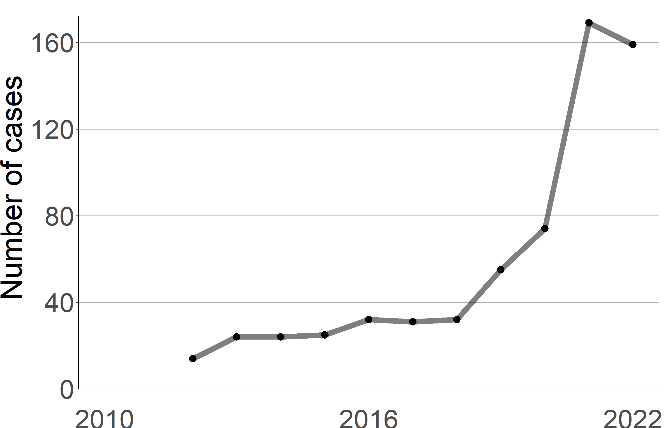
5. The header and footer
The final two pieces of the table are the header and footer. The header consists of a main title and a subtitle with a brief table description; the footer shows the data source of the species images and descriptions. Again, the text is written in HTML to allow for more customization.
title_text <- "<b><i>Top Ten Bird-Window Collision Species in Taiwan</i></b>"

subtitle_text <- "This summary table shows the top ten bird-window collision
species between 2010 and 2022 in Taiwan, based on a data set collected from
<span style = 'color: #ffc107'>The Taiwan Roadkill Observation Network</span> and
<span style = 'color: #4267B2'>Reports on Bird-Glass Collisions Facebook Group</span>.
170 species with around 3,600 collision cases were recorded over this 13-year period."

footer_text <- "<p margin-bottom: 0em><i>Species images and descriptions:
The Cornell Lab of Ornithology Macaulay Library & eBird</i> <span style = 'margin-left: 5px'> <img src = 'https://raw.githubusercontent.com/GenChangHSU/ggGallery/master/_posts/2023-02-18-post-24-gt-and-ggplot-visualizing-bwc-in-taiwan/Macaulay_lib_logo.png' width = '90' height = '30' style = 'vertical-align: middle'/></span><span style = 'margin-left: 3px'><img src = 'https://raw.githubusercontent.com/GenChangHSU/ggGallery/master/_posts/2023-02-18-post-24-gt-and-ggplot-visualizing-bwc-in-taiwan/eBird_logo.png' width = '70' height = '30' style = 'vertical-align: middle'/></p>"
6. Put everything together
Having all the ingredients on hand, it’s time to put them together! There are several things to note here:
We prepare a data frame with the columns in the desired order and pass it to the master function
gt()to create a table.We create two blank columns to add some white space. The amount of spacing may not be desirable now, but this can be easily adjusted later.
We use the function
gt_img_circle()to create circle images of the species.Remember we used HTML in the short descriptions? This is not readily recognized by
gt(), but we can usetext_transform()along withhtml()to tellgt()that the column “description” should be understood in the HTML language.For the line charts, we first set the column elements to NA, and again use
text_transform()along withggplot_image()to tellgt()that the line charts in the list “bwc_linecharts” should be treated as ggplots.Same as the descriptions, the header and footer are passed into
html()so that the text is understood in the HTML language.
library(gt)
library(gtExtras)  # for the function gt_img_circle()

### Build the first table
bwc_table <- bwc_top_collision_df %>%
  mutate(blank1 = "", blank2 = "", linechart = NA) %>%
  select(blank1, image, blank2, description, n, linechart) %>%
  gt() %>%

  # images
  gt_img_circle(column = "image", height = 100, border_weight = 0) %>%

  # short descriptions
  text_transform(locations = cells_body(columns = description),
                 fn = function(x){map(bwc_top_collision_df$description, html)}) %>%

  # line charts
  text_transform(locations = cells_body(columns = linechart),
                 fn = function(x){map(bwc_linecharts, ggplot_image,
                                      height = px(90), aspect_ratio = 2.2)}) %>%
  # header
  tab_header(title = html(title_text),
             subtitle = html(subtitle_text)) %>%

  # footer
  tab_source_note(source_note = html(footer_text))

bwc_table| Top Ten Bird-Window Collision Species in Taiwan | |||||
| This summary table shows the top ten bird-window collision species between 2010 and 2022 in Taiwan, based on a data set collected from The Taiwan Roadkill Observation Network and Reports on Bird-Glass Collisions Facebook Group. 170 species with around 3,600 collision cases were recorded over this 13-year period. | |||||
| blank1 | image | blank2 | description | n | linechart |
|---|---|---|---|---|---|
Taiwan barbet (Psilopogon nuchalis)
|
639 |  | |||
Asian emerald dove (Chalcophaps indica)
|
351 |  | |||
Spotted dove (Streptopelia chinensis)
|
196 |  | |||
Eurasian tree sparrow (Passer montanus)
|
193 |  | |||
Crested goshawk (Accipiter trivirgatus)
|
188 |  | |||
Common kingfisher (Alcedo atthis)
|
176 |  | |||
Light-vented bulbul (Pycnonotus sinensis)
|
155 |  | |||
Pale thrush (Turdus pallidus)
|
144 |  | |||
Swinhoe's white-eye (Zosterops simplex)
|
97 |  | |||
Oriental turtle dove (Streptopelia orientalis)
|
93 |  | |||
Species images and descriptions:
The Cornell Lab of Ornithology Macaulay Library & eBird |
|||||
Nice, we get our fist table out! Though, it is not in a good shape and definitely needs some adjustments and fine-tuning. This is what we are going to do next.
7. Polish the table
There are quite a few things in the table we can modify:
Column labels
Column widths
Table width and the padding around table components
The style (font size, font family, color, alignment, etc.) of header, column labels, body columns, and footer
The background color of the table rows
The main purpose here is to show that we can customize the table as we wish, and so I’ll not dive into the nitty-gritty of styling functions and arguments. In fact, we are only scratching the surface, and there are a lot more things we can do. If interested, check out the amazing references and tutorials on the gt package website for more details!
It does require a bit of trial and error to get everything at the exact place. So be patient and have fun experimenting. It’s super satisfying to see the final product!
bwc_table <- bwc_table %>%
# column labels
cols_label(blank1 = "",
image = "",
blank2 = "",
description = "",
n = html("2010-2022 <br> Total Cases"),
linechart = html("2010-2022 <br> Annual Trend")) %>%
# column widths
cols_width(blank1 ~ px(10),
image ~ px(107.5),
blank2 ~ px(10),
description ~ px(370),
n ~ px(110),
linechart ~ px(300)) %>%
# table width and padding
tab_options(table.width = 900,
container.width = 950,
heading.padding = px(12),
data_row.padding = px(0),
source_notes.padding = px(0)) %>%
# title style
tab_style(locations = cells_title(groups = "title"),
style = list(cell_text(font = google_font(name = "Kanit"),
size = px(35),
align = "left"))) %>%
# subtitle style
tab_style(locations = cells_title(groups = "subtitle"),
style = list(cell_text(font = google_font(name = "Arimo"),
size = px(20),
color = "grey30",
align = "left"))) %>%
# column label style
tab_style(locations = cells_column_labels(c(n, linechart)),
style = list(cell_text(font = google_font(name = "Arimo"),
v_align = "middle",
weight = "bold",
size = "large"))) %>%
# body column style
tab_style(locations = cells_body(columns = c(description)),
style = list(cell_text(font = google_font(name = "Arimo"),
align = "center"))) %>%
tab_style(locations = cells_body(columns = c(n)),
style = list(cell_text(font = google_font(name = "Arimo"),
align = "center",
size = px(25)))) %>%
# footer style
tab_style(locations = cells_source_notes(),
style = list(cell_text(font = google_font(name = "Arimo"),
size = "small",
v_align = "top"))) %>%
# row background color
tab_style(locations = cells_body(rows = seq(1, 10, 2)),
style = list(cell_fill(color = "#d8dde0")))
bwc_table| Top Ten Bird-Window Collision Species in Taiwan | |||||
| This summary table shows the top ten bird-window collision species between 2010 and 2022 in Taiwan, based on a data set collected from The Taiwan Roadkill Observation Network and Reports on Bird-Glass Collisions Facebook Group. 170 species with around 3,600 collision cases were recorded over this 13-year period. | |||||
| 2010-2022 Total Cases |
2010-2022 Annual Trend |
||||
|---|---|---|---|---|---|
Taiwan barbet (Psilopogon nuchalis)
|
639 | | |||
Asian emerald dove (Chalcophaps indica)
|
351 | | |||
Spotted dove (Streptopelia chinensis)
|
196 | | |||
Eurasian tree sparrow (Passer montanus)
|
193 | | |||
Crested goshawk (Accipiter trivirgatus)
|
188 | | |||
Common kingfisher (Alcedo atthis)
|
176 | | |||
Light-vented bulbul (Pycnonotus sinensis)
|
155 | | |||
Pale thrush (Turdus pallidus)
|
144 | | |||
Swinhoe's white-eye (Zosterops simplex)
|
97 | | |||
Oriental turtle dove (Streptopelia orientalis)
|
93 | | |||
Species images and descriptions:
The Cornell Lab of Ornithology Macaulay Library & eBird |
|||||
Looks cool, but still there are a few formatting issues (e.g., the short descriptions are cut off on the right) when displayed as an HTML page here.
We can save the HTML as an image to solve this problem:
library(webshot2)
gtsave_extra(bwc_table, "bwc_table.png", zoom = 2)
This is the final table. Perfect!

8. The messages from the table
Before we call it a wrap, let’s take a closer look at the table and see what we can learn from it.
Many of the bird species on the list commonly occur in urban or sub-urban areas (e.g., spotted dove, Eurasian tree sparrow, light-vented bulbul, Swinhoe’s white-eye, and oriental turtle dove), which is a strong reason why they collide with windows quite frequently. But the collision issue is not limited to urban dwellers. There is also common kingfisher, a species that lives around water bodies, and pale thrush, a winter migrant in Taiwan. In fact, nine of the top ten species are resident birds, even though Taiwan lies close to the center of the East Asian-Australian Flyway. This is quite different from the patterns in the Western countries, where the majority of collisions are migratory birds.
The species that tops the list, Taiwan barbet (an endemic species in Taiwan), has nearly twice as many collision cases as the second species! This is quite special as not many cases have been reported for similar species in other countries. Another surprising species on the list is the raptor crested goshawk. It’s a bit mind-boggling that such an agile flyer also falls victim to bird-window collision. This could potentially have some ecological impacts as hawks are top predators in the ecosystem. Interestingly, three dove species show up on the list. Perhaps it’s because they are relatively poor in maneuvering, and also they are quite abundant around human settlements. A combination of both makes them vulnerable to window collisions.
In general, the collisions for these top ten species are trending upwards, despite some year-to-year fluctuations. This may be due to more reports in recent years as people are more aware of bird-window collisions. It can also be that there are more buildings/infrastructures with window surface, thus causing more collisions. The increasing trends are concerning and deserve our close attention.
It is noteworthy that the numbers of total cases shown in the table are just the tip of the iceberg: A majority of bird-window collisions got unnoticed. Even if noticed, many were unreported. There is increasing research on why birds collide with windows, and hopefully we will come up with effective measures to prevent it.
Summary
To recap, in this post we built a cool gt table to visualize the top ten bird-window collision species in Taiwan. We first prepared the table columns, then put them in a data frame and created a first table, and finally polished the table by tweaking the format and style. We also integrated ggplots into the table to enhance data visualization.
I used to think that R is not good at making tables, but now I’ve completely changed my point of view after writing this post. I believe you will have an itch for making your own gt tables too!
Hope you learn something useful from this post and don’t forget to leave your comments and suggestions below if you have any!
Loss, S. R., Will, T., & Marra, P. P. (2015). Direct mortality of birds from anthropogenic causes. Annual Review of Ecology, Evolution, and Systematics, 46, 99-120.↩︎
