The problem
Suppose that we want to visualize the relationship (i.e., a scatterplot) between engine displacement (displ) and highway miles per gallon (hwy) of cars in the mpg dataset. And for some reason, we would like to create separate figures for each of the three drive train types (drv) rather than having a single figure with three panels (i.e., facets). Also, the data points in the figures will be colored by car type (class).
library(tidyverse)

# Four-wheel drive
plot_drv4 <- mpg %>%
  mutate(class = factor(class)) %>%
  filter(drv == "4") %>%
  ggplot(aes(x = displ, y = hwy)) +
  geom_point(aes(color = class)) +
  stat_smooth(method = "lm", se = F) +
  lims(x = c(1, 7), y = c(10, 30)) +
  labs(title = "Four-wheel drive") +
  theme_classic() +
  theme(plot.title = element_text(size = 12, hjust = 0.5),
        legend.title.align = 0.5)

# Front-wheel drive
plot_drvf <- mpg %>%
  mutate(class = factor(class)) %>%
  filter(drv == "f") %>%
  ggplot(aes(x = displ, y = hwy)) +
  geom_point(aes(color = class)) +
  stat_smooth(method = "lm", se = F) +
  lims(x = c(1, 6), y = c(10, 45)) +
  labs(title = "Front-wheel drive") +
  theme_classic() +
  theme(plot.title = element_text(size = 12, hjust = 0.5),
        legend.title.align = 0.5)

# Rear wheel drive
plot_drvr <- mpg %>%
  mutate(class = factor(class)) %>%
  filter(drv == "r") %>%
  ggplot(aes(x = displ, y = hwy)) +
  geom_point(aes(color = class)) +
  stat_smooth(method = "lm", se = F) +
  lims(x = c(3, 7.5), y = c(10, 30)) +
  labs(title = "Rear-wheel drive") +
  theme_classic() +
  theme(plot.title = element_text(size = 12, hjust = 0.5),
        legend.title.align = 0.5)

plot_drv4
plot_drvf
plot_drvr


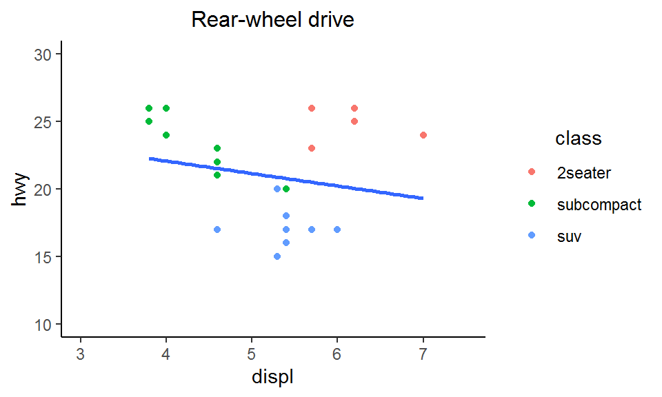
Have you spotted something weird? Yup, the colors of the levels in class are not consistent across the three figures (e.g., salmon red represents “compact” in the first two figures but “2seater” in the third; “subcompact” has three different colors in the three figures!) This problem arises because some factor levels are shared across (two or all three) figures while the others are missing, and by default ggplot will only color the levels appearing in the data and omit the rest.
The partial solution
So how can you fix this problem? Well, there is a workaround: since ggplot by default omits the unused levels, we can ask ggplot not to do so by specifying drop = F in scale_color_XXX():
# Four-wheel drive
plot_drv4_undropped <- mpg %>%
  mutate(class = factor(class)) %>%
  filter(drv == "4") %>%
  ggplot(aes(x = displ, y = hwy)) +
  geom_point(aes(color = class)) +
  scale_color_discrete(drop = F) +  # Not to drop the unused levels
  stat_smooth(method = "lm", se = F) +
  lims(x = c(1, 7), y = c(10, 30)) +
  labs(title = "Four-wheel drive") +
  theme_classic() +
  theme(plot.title = element_text(size = 12, hjust = 0.5),
        legend.title.align = 0.5)

# Front-wheel drive
plot_drvf_undropped <- mpg %>%
  mutate(class = factor(class)) %>%
  filter(drv == "f") %>%
  ggplot(aes(x = displ, y = hwy)) +
  geom_point(aes(color = class)) +
  scale_color_discrete(drop = F) +
  stat_smooth(method = "lm", se = F) +
  lims(x = c(1, 6), y = c(10, 45)) +
  labs(title = "Front-wheel drive") +
  theme_classic() +
  theme(plot.title = element_text(size = 12, hjust = 0.5),
        legend.title.align = 0.5)

# Rear wheel drive
plot_drvr_undropped <- mpg %>%
  mutate(class = factor(class)) %>%
  filter(drv == "r") %>%
  ggplot(aes(x = displ, y = hwy)) +
  geom_point(aes(color = class)) +
  scale_color_discrete(drop = F) +
  stat_smooth(method = "lm", se = F) +
  lims(x = c(3, 7.5), y = c(10, 30)) +
  labs(title = "Rear-wheel drive") +
  theme_classic() +
  theme(plot.title = element_text(size = 12, hjust = 0.5),
        legend.title.align = 0.5)

plot_drv4_undropped
plot_drvf_undropped
plot_drvr_undropped

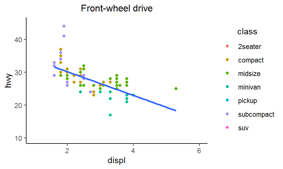

Now, as you can see, each level in class is associated with a specific color across all three figures. However, another problem comes (I bet you already know what it is): the unused levels are shown in the legends even though they do not appear in the plots (e.g., there is no “2seater” car with four-wheel drive, but “2seater” still shows up in the legend). Depending on the nature of your figure and your purpose, if the legends are not necessary, you can simply hide them while having consistent colors across the figures. But what if you want to keep the legends? Keep reading!
The ultimate solution
So what is the ultimate solution to this problem? Three steps:
First, create a named vector with colors (can be either hex color codes, color names, or a mixture of them) as the vector elements and factor levels as their names. Note that all levels of the factor across the figures should appear as the vector names, which means the length of the vector should be the same as the number of factor levels. This named vector will be the palette for the next step.
Next, use scale_color_manual(values = name_of_palette) to manually set the colors of the factor levels based on the palette.
Finally, identify the subset of factor levels appearing in the data you are using for that specific figure and specify them using the argument limits = in scale_color_manual().
Okay, to see is to believe. Here is a demo:
library(RColorBrewer)

# Create a named vector as the palette
class <- unique(mpg$class)  # All factor levels across figures
colors <- brewer.pal(length(class), "Set1")  # Colors
my_palette <- set_names(colors, class)  # Named vector

# Four-wheel drive
class_drv4 <- mpg %>%
  filter(drv == "4") %>%
  .$class %>%
  unique()  # Subset of levels in "class" for four-wheel drive cars

plot_drv4_manual <- mpg %>%
  mutate(class = factor(class)) %>%
  filter(drv == "4") %>%
  ggplot(aes(x = displ, y = hwy)) +
  geom_point(aes(color = class)) +
  scale_color_manual(values = my_palette, limits = class_drv4) +  # Manually set the colors of the factor levels based on the palette and also specify the levels present in the data
  stat_smooth(method = "lm", se = F) +
  lims(x = c(1, 7), y = c(10, 30)) +
  labs(title = "Four-wheel drive") +
  theme_classic() +
  theme(plot.title = element_text(size = 12, hjust = 0.5),
        legend.title.align = 0.5)

# Front-wheel drive
class_drvf <- mpg %>%
  filter(drv == "f") %>%
  .$class %>%
  unique()

plot_drvf_manual <- mpg %>%
  mutate(class = factor(class)) %>%
  filter(drv == "f") %>%
  ggplot(aes(x = displ, y = hwy)) +
  geom_point(aes(color = class)) +
  scale_color_manual(values = my_palette, limits = class_drvf) +
  stat_smooth(method = "lm", se = F) +
  lims(x = c(1, 6), y = c(10, 45)) +
  labs(title = "Front-wheel drive") +
  theme_classic() +
  theme(plot.title = element_text(size = 12, hjust = 0.5),
        legend.title.align = 0.5)

# Rear wheel drive
class_drvr <- mpg %>%
  filter(drv == "r") %>%
  .$class %>%
  unique()

plot_drvr_manual <- mpg %>%
  mutate(class = factor(class)) %>%
  filter(drv == "r") %>%
  ggplot(aes(x = displ, y = hwy)) +
  geom_point(aes(color = class)) +
  scale_color_manual(values = my_palette, limits = class_drvr) +
  stat_smooth(method = "lm", se = F) +
  lims(x = c(3, 7.5), y = c(10, 30)) +
  labs(title = "Rear-wheel drive") +
  theme_classic() +
  theme(plot.title = element_text(size = 12, hjust = 0.5),
        legend.title.align = 0.5)

plot_drv4_manual
plot_drvf_manual
plot_drvr_manual


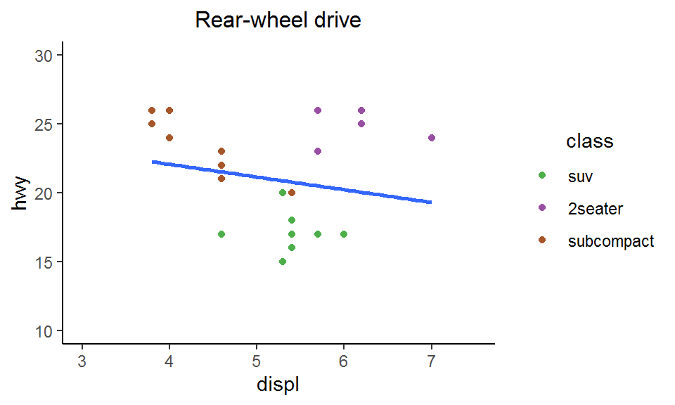
Now, not only are the colors of the factor levels consistent across the figures, but also the legends are properly displaying the levels appearing in the plots. Problem solved!
An advantage of this approach is that it offers great flexibility for users to select the colors they would like for each factor level. Of course, you have to spend a bit of time creating the palette yourself instead of just lazily asking ggplot to automatically color the levels for you. But think in the other way round: you get 100% control of the colors! Doesn’t that sound good?
Last but not least, in this example I used the built-in color palette “Set1” from the package RColorBrewer, which provides different types of palettes coming in a variety of colors. And if you want to build your own palette from scratch, definitely check out the website ColorBrewer. There are tons of options to customize the colors to your heart’s content.
That’s it for this post and don’t forget to leave your comments and suggestions below if you have any. Also, do let me know if you find another (perhaps even simpler) way to do the same job!
