This vignette shows you some examples of using the package’s main function, create_pal. You will learn how to make good use of its functionality to create your own awesome palette.

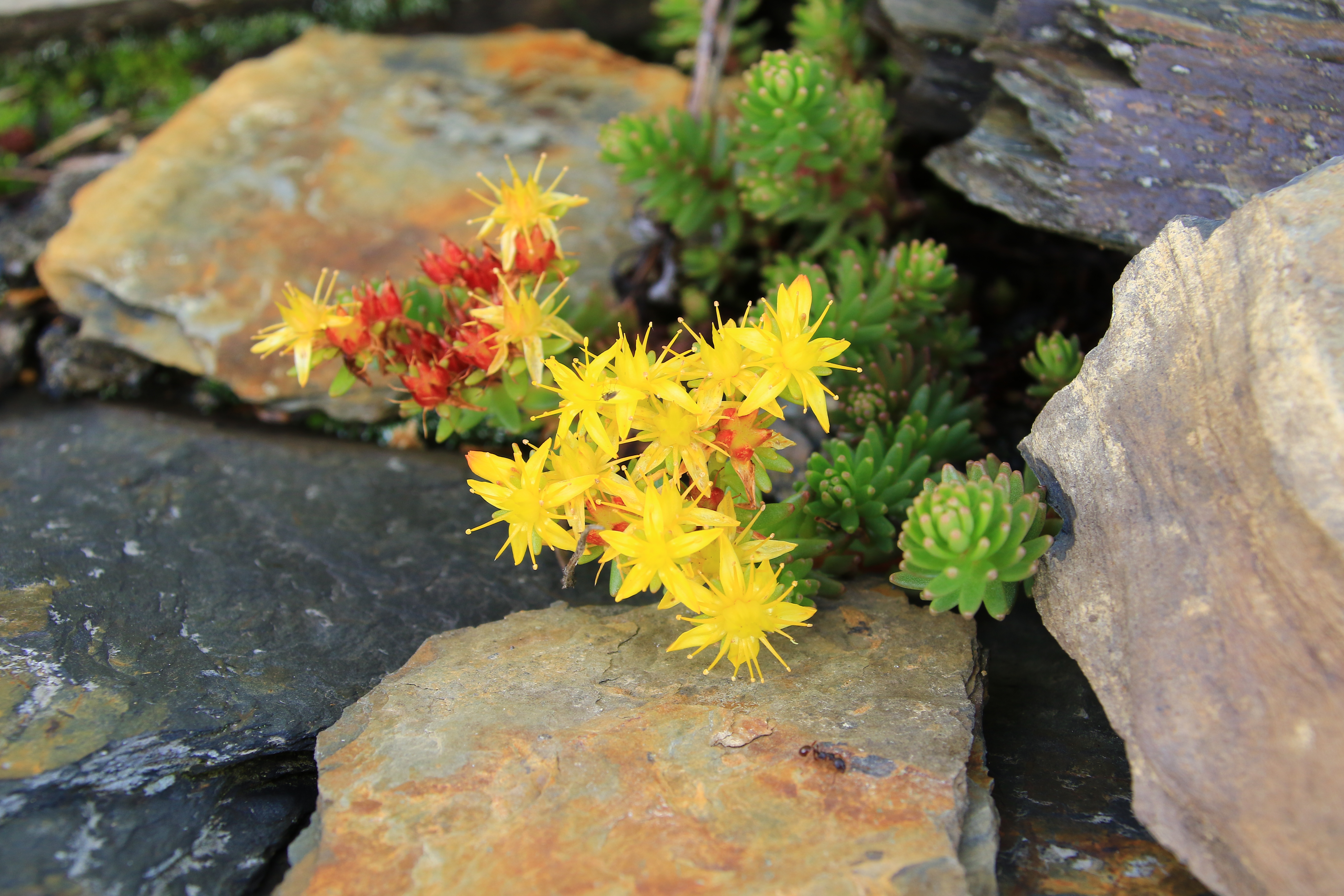
We will play around with the create_pal function using the image below (photo credit: Gen-Chang Hsu). This stonecrop species (Sedum morrisonense Hayata) is endemic to Taiwan and commonly seen at mid- and high-altitudes. It thrives in the rock cracks and crevices, growing low and spreading out to avoid strong wind. It is also characterized by its densely-clumped, fingernail-like succulent leaves, which are used for water storage in addition to photosynthesis. During summertime, blossoms of bright yellow flowers will burst into bloom.

Part 1. Create the Palette

Now let’s start with a simple example:

# Get the path of the image
library(PalCreatoR)
image_path <- system.file("Alpine Flower.JPG", package = "PalCreatoR")

# Create a basic palette with 5 colors
My_pal_5 <- create_pal(image = image_path, n = 5, title = "My Palette (n = 5)")

print(My_pal_5)
#> [1] "#8B7E61" "#4E5542" "#EDCB37" "#212218" "#BAA586"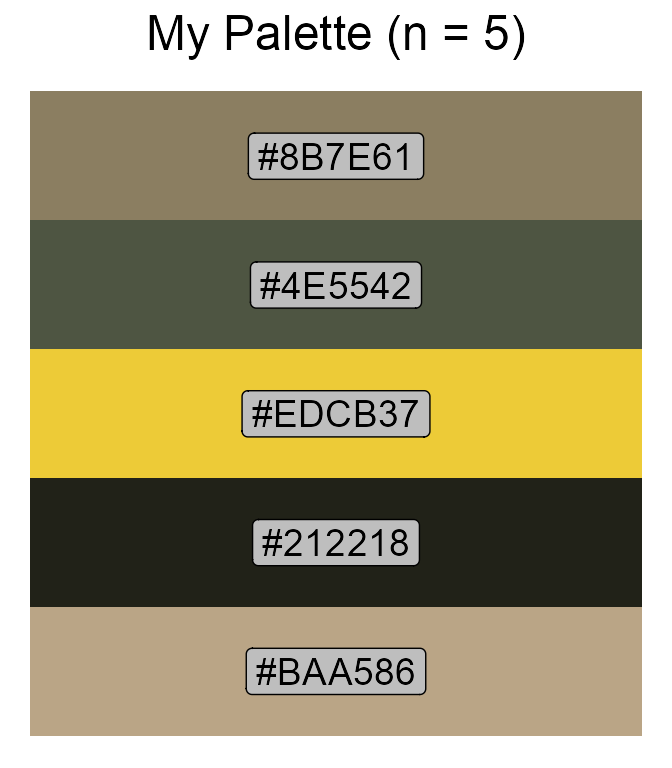

More colors:

My_pal_10 <- create_pal(image = image_path, n = 10, title = "My Palette (n = 10)")

print(My_pal_10)
#>  [1] "#A98149" "#777570" "#F1D135" "#3A3E29" "#CBBEA5" "#171811" "#4D5252"
#>  [8] "#C4A56F" "#A89985" "#64772F"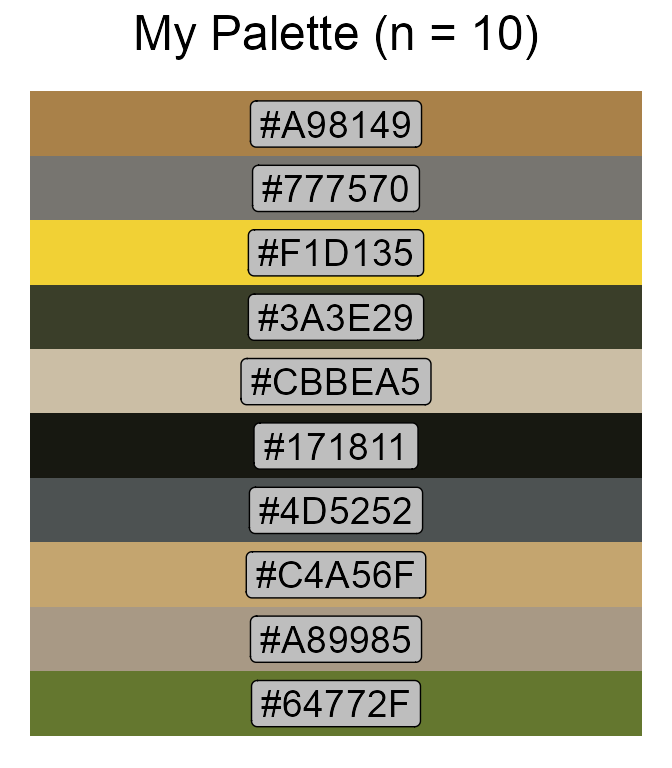

By default, the colors in the palette are not checked for colorblind safe. To get the colorblind-friendly colors, set colorblind = TRUE:

My_pal_clb <- create_pal(image = image_path, n = 5, colorblind = TRUE, 
    title = "My Palette \n (colorblind-friendly)")

print(My_pal_clb)
#> [1] "#8B7E60" "#435E6A" "#00D9FF" "#19252D" "#BCA681"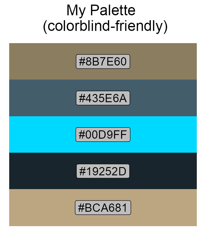

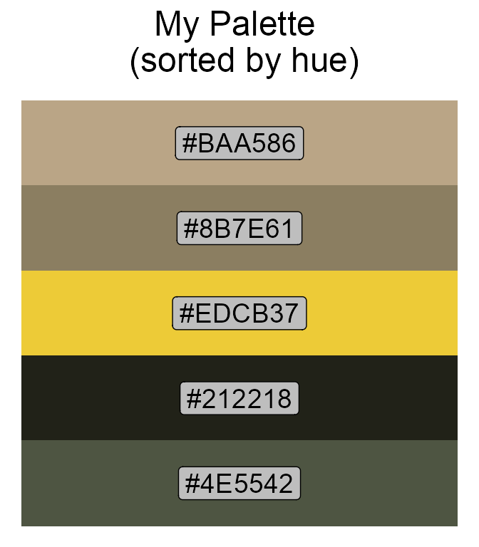
The colors in the palette are not ordered by default. You can sort the colors in the HSV color space. Three options are available:

sort = "hue": the colors are sorted by hue ¹ in an ascending order (i.e., from red, yellow, green, to cyan, blue, and magenta);
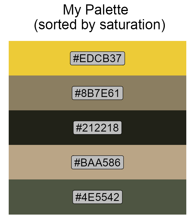
sort = "saturation": the colors are sorted by saturation ² in a descending order (i.e., from pure to gray);
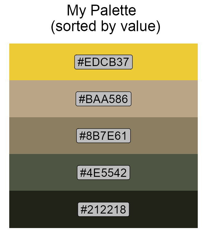
sort = "value": the colors are sorted by value ³ in a descending order (i.e., from bright to dark).

Let’s visualize the effects of color sorting:

# Unsorted
My_pal_none <- create_pal(image = image_path, n = 5, sort = "none", 
    title = "My Palette \n (unsorted)")

# By hue
My_pal_hue <- create_pal(image = image_path, n = 5, sort = "hue", 
    title = "My Palette \n (sorted by hue)")

# By saturation
My_pal_saturation <- create_pal(image = image_path, n = 5, sort = "saturation", 
    title = "My Palette \n (sorted by saturation)")

# By value
My_pal_value <- create_pal(image = image_path, n = 5, sort = "value", 
    title = "My Palette \n (sorted by value)")

Another novel feature in the create_pal function is that you can specify method = "Gaussian_mix" to apply multivariate Gaussian mixture modeling (GMM) instead of the default kmeans algorithm to extract the representative colors from the image:

# kmeans
My_pal_kmeans <- create_pal(image = image_path, n = 5, method = "kmeans", 
    sort = "value", title = "My Palette \n (kmeans)")

# Gaussian mixture modeling
My_pal_Gaussian_mix <- create_pal(image = image_path, n = 5, 
    method = "Gaussian_mix", sort = "value", title = "My Palette \n (GMM)")

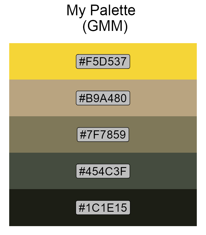
Not much difference in this case.

By the way, if you do not want to see your palette, set show.pal = FALSE. This will return only the color code vector.

Part 2. Modify the Palette

You can modify the alpha transparency⁴ of the colors in the palette using the helper function modify_pal. Simply pass the palette and a vector of alpha values into the function, and you will get the modified colors!

# Original palette
My_pal <- create_pal(image = image_path, n = 5, method = "kmeans", 
    sort = "value", title = "My Palette")

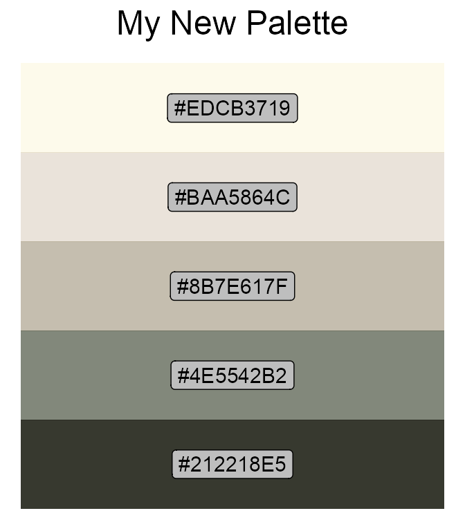
# Modified palette
My_new_pal <- modify_pal(pal = My_pal, alpha = c(0.1, 0.3, 0.5, 
    0.7, 0.9), title = "My New Palette")

In general, the number of colors in the palette and the number of alpha values should be the same. Any extra elements in the longer vector will be omitted to match the elements in the shorter one. However, there are two exceptions:

A single color + multiple alpha values: If you have a single color but pass multiple alpha values to the function, then you will get a sequence of that color with different transparencies. This is useful for generating a color gradient.

My_col_gradient <- modify_pal(pal = My_pal[1], alpha = c(0.1, 
    0.3, 0.5, 0.7, 0.9), title = "My Color Gradient")

print(My_col_gradient)
#> [1] "#EDCB3719" "#EDCB374C" "#EDCB377F" "#EDCB37B2" "#EDCB37E5"

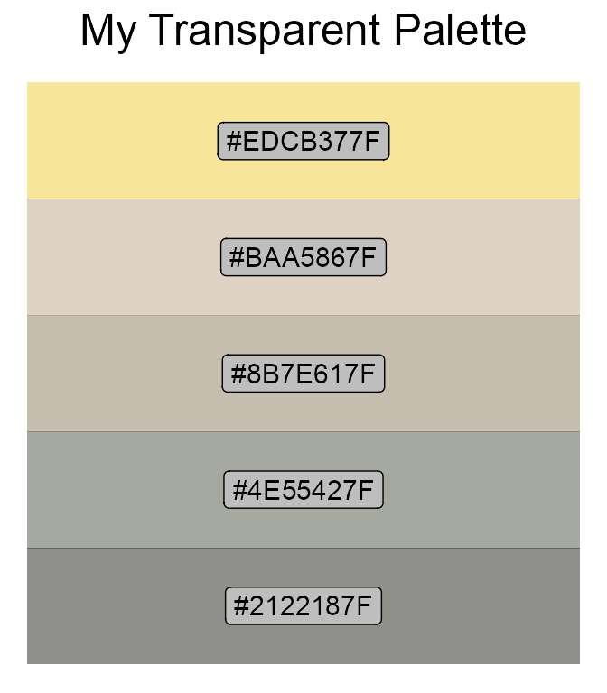
Multiple colors + a single alpha value: If you have multiple colors but pass only a single alpha value to the function, then all the colors will be adjusted by the same degree of transparency. This is useful for toning down the palette colors in a uniform manner.


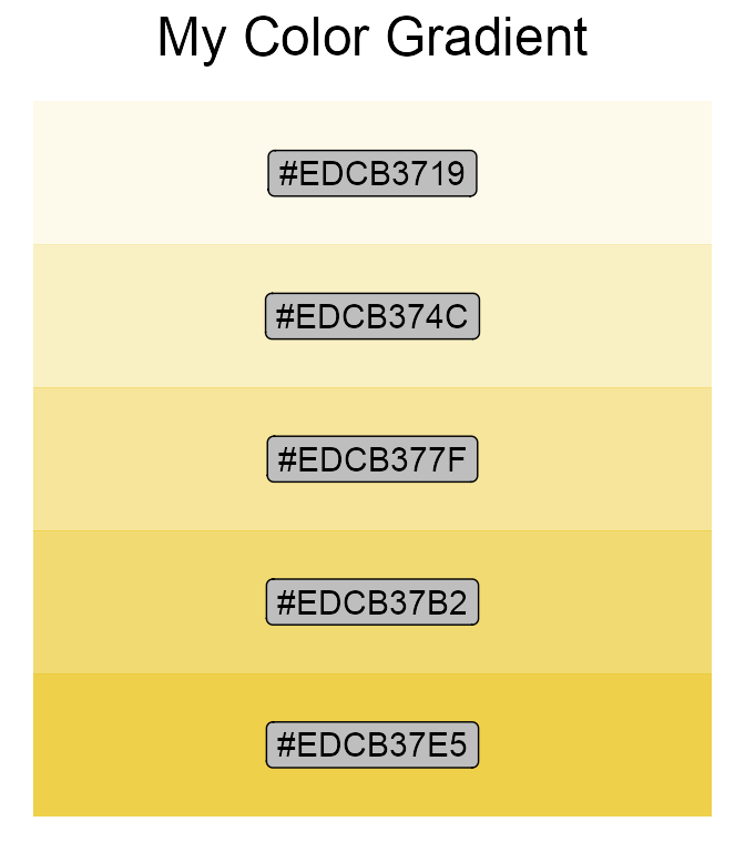
My_pal <- create_pal(image = image_path, n = 5, method = "kmeans", 
    sort = "value", title = "My Palette")

My_trans_pal <- modify_pal(pal = My_pal, alpha = 0.5, title = "My Transparent Palette")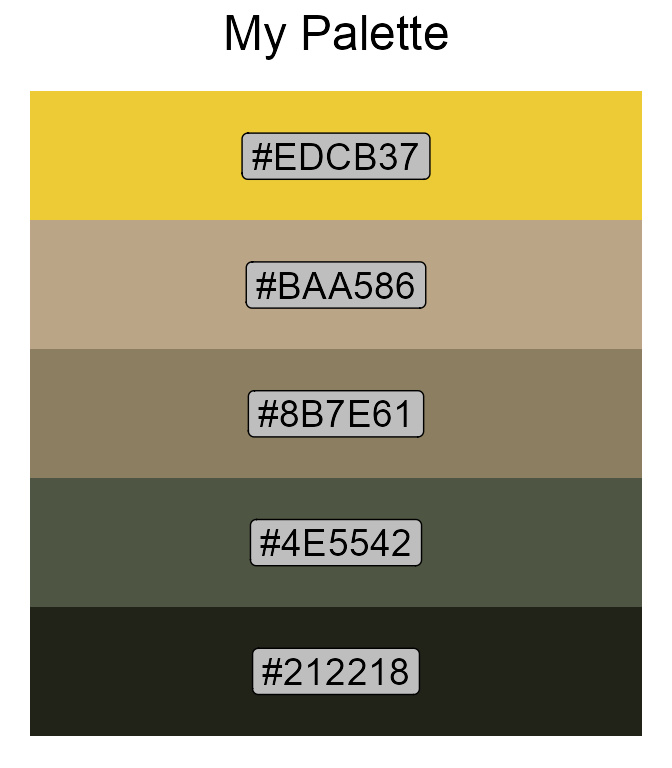

Of course, the color palette you pass to the pal argument does not necessarily have to be generated from the create_pal function. You can specify any color you want as long as they are in hexadecimal color format!

Part 3. Use the Palette

Finally, let’s use the palettes in the real figures:

library(ggplot2)
library(ggpubr)

# Create the palettes
My_pal1 <- create_pal(image = image_path, n = 10, sort = "value", colorblind = FALSE, show.pal = F)
My_pal2 <- create_pal(image = image_path, n = 10, sort = "value", colorblind = TRUE, show.pal = F)

# The golden spiral
spiral_df <- data.frame(x = seq(0, 13, length.out = 5000)) %>%
  mutate(y = exp(0.30635*x)) %>%
  mutate(x = rev(x),
         y = rev(y),
         polar_x = y*cos(x),
         polar_y = y*sin(x),
         x_start = rep(0, 5000),
         y_start = rep(0, 5000))

# Plot the spirals (package logo)
spiral_p1 <- ggplot(spiral_df) +
  geom_segment(aes(x = x_start, y = y_start, xend = polar_x, yend = polar_y),
               color = rep(My_pal1, each = 500),
               size = 1) +
  geom_point(aes(x = polar_x, y = polar_y),
             color = "black",
             size = 0.1) +
  coord_fixed(ratio = 1) +
  theme_void()

spiral_p2 <- ggplot(spiral_df) +
  geom_segment(aes(x = x_start, y = y_start, xend = polar_x, yend = polar_y),
               color = rep(My_pal2, each = 500),
               size = 1) +
  geom_point(aes(x = polar_x, y = polar_y),
             color = "black",
             size = 0.1) +
  coord_fixed(ratio = 1) +
  theme_void()

# Arrange the spirals
ggarrange(spiral_p1, spiral_p2)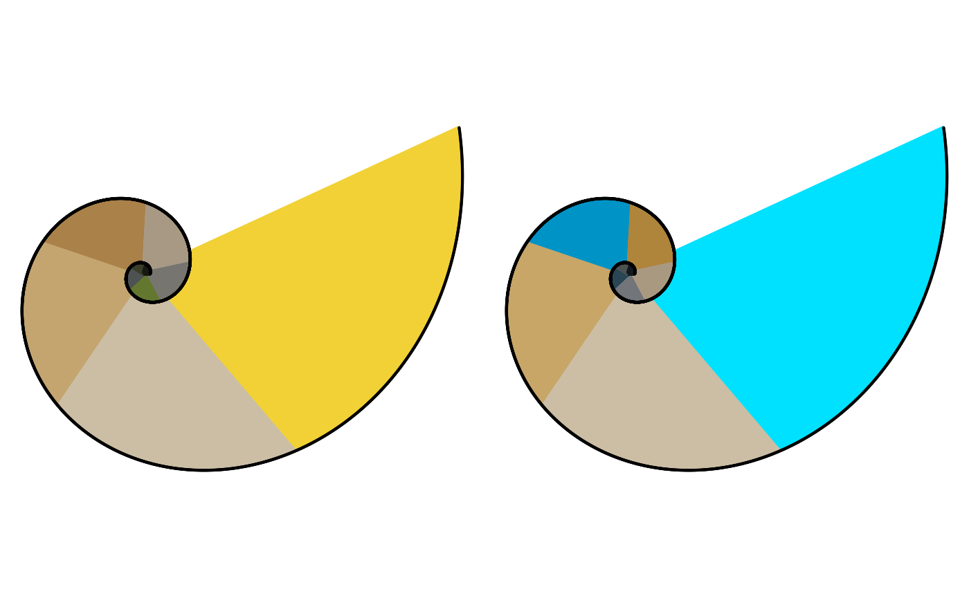

# Dazzling effect
spiral_p1_dazzle <- ggplot(spiral_df) +
  geom_segment(aes(x = x_start, y = y_start, xend = polar_x, yend = polar_y),
               color = rep(My_pal1, 500),
               size = 1) +
  geom_point(aes(x = polar_x, y = polar_y),
             color = "black",
             size = 0.1) +
  coord_fixed(ratio = 1) +
  theme_void()

spiral_p2_dazzle <- ggplot(spiral_df) +
  geom_segment(aes(x = x_start, y = y_start, xend = polar_x, yend = polar_y),
               color = rep(My_pal2, 500),
               size = 1) +
  geom_point(aes(x = polar_x, y = polar_y),
             color = "black",
             size = 0.1) +
  coord_fixed(ratio = 1) +
  theme_void()

# Arrange the spirals
ggarrange(spiral_p1_dazzle, spiral_p2_dazzle)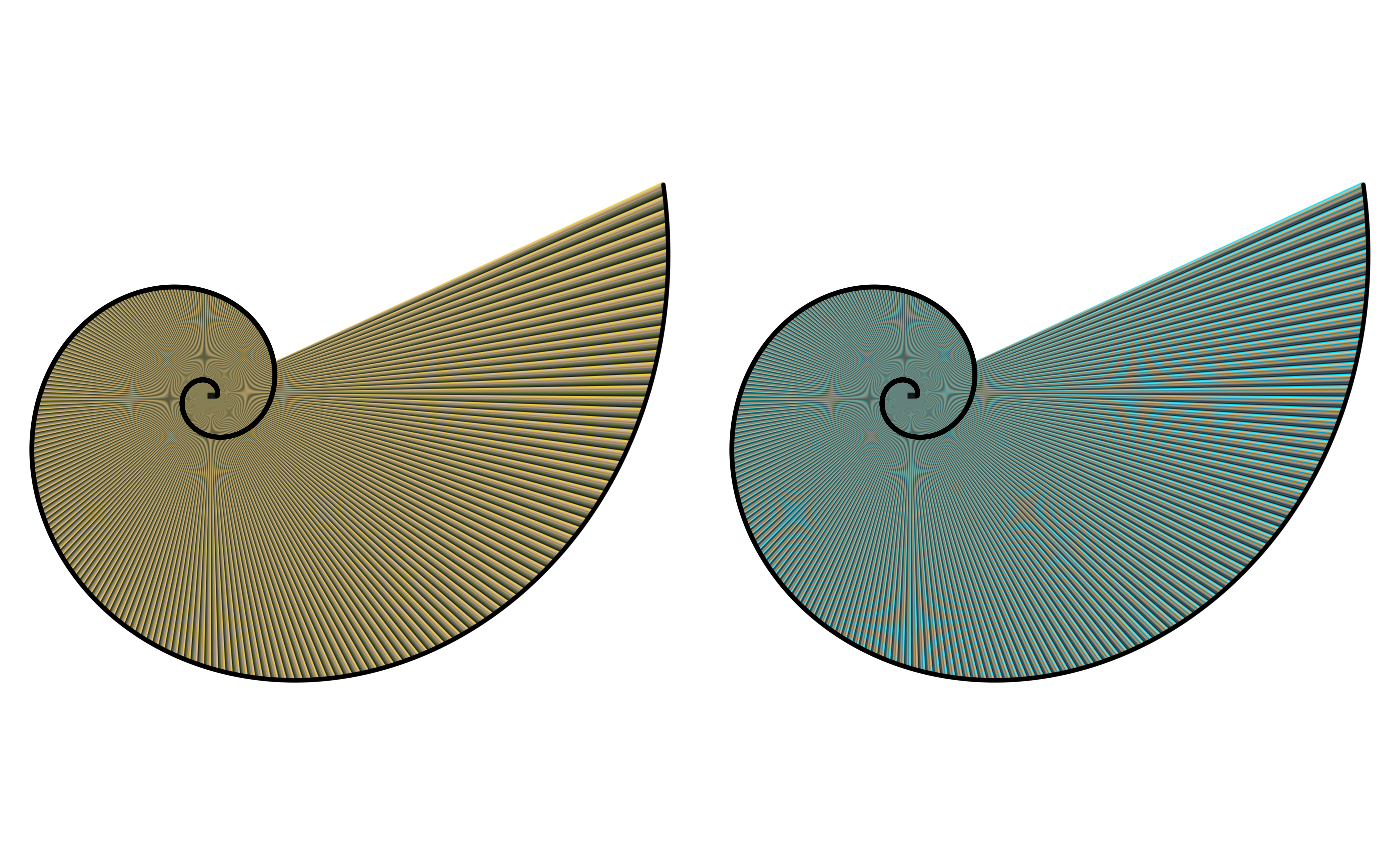

# Continuous color spectrum
My_pal3 <- create_pal(image = image_path, n = 5000, sort = "value", colorblind = FALSE, show.pal = F) 
# This might take a while to run

spiral_p3 <- ggplot(spiral_df) +
  geom_segment(aes(x = x_start, y = y_start, xend = polar_x, yend = polar_y),
               color = rep(My_pal3),
               size = 1) +
  geom_point(aes(x = polar_x, y = polar_y),
             color = "black",
             size = 0.1) +
  coord_fixed(ratio = 1) +
  theme_void()

spiral_p3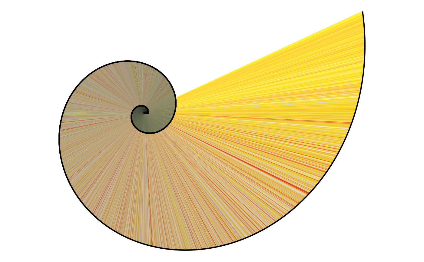

# Color gradients with different alpha transparencies
My_pal4 <- create_pal(image = image_path, n = 5, sort = "value", colorblind = FALSE, show.pal = F) 

My_new_pal <- modify_pal(pal = My_pal4[1], alpha = seq(0.1, 1.0, 0.1), show.pal = F)

spiral_new_pal <- ggplot(spiral_df) +
  geom_segment(aes(x = x_start, y = y_start, xend = polar_x, yend = polar_y),
               color = rep(My_new_pal, each = 500),
               size = 1) +
  geom_point(aes(x = polar_x, y = polar_y),
             color = "black",
             size = 0.1) +
  coord_fixed(ratio = 1) +
  theme_void()

spiral_new_pal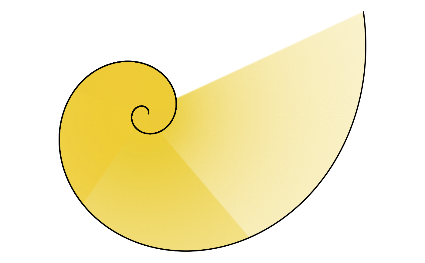

Interested? Grab your own image and try it out now!

Have fun and enjoy!!!

Hue represents the angle of the color (in degree) on the RGB color circle. A hue value of 0° gives red, 120° green, and 240° blue.↩︎
Saturation controls the amount of color used. A saturation value of 100% will be the purest color possible for the given hue; a saturation value of 0% results in grayscale color.↩︎
Value indicates the brightness of the color. A value of 100% has no black mixed into the color; a value of 0% gives pure black.↩︎
An alpha value defines the “transparency”, or “opacity” of the color. A value of 0 means completely transparent (i.e., the background will completely “show through”); a value of 1 means completely opaque (i.e., none of the background will “show through”). In short, the lower the alpha value is, the lower “amount” of the color will be.↩︎

Quick Demonstration

Part 1. Create the Palette

Part 2. Modify the Palette

Part 3. Use the Palette